
How to plan fiber optic cabling for a data center: MDA/HDA zones, topology, backbone fiber grades, fiber counts, link budgets, cords, adapters, pathways, testing and ordering — with typical figures subject to datasheet.

Fiber optic cabling is the layer of a data center that everything else depends on. Switches, servers and storage get replaced every few years; the cabling that connects them is expected to stay in place for a decade or more. That mismatch in lifecycle is the reason cabling deserves its own planning pass before any equipment order is placed. When the cabling plan is skipped, projects pay for it later in re-pulled runs, oversized transceiver costs, airflows blocked by cable spaghetti, and links that pass a continuity check at commissioning but show errors under production load. When the cabling plan is done properly, the same physical infrastructure supports several generations of equipment upgrades without a disruptive rebuild.
This guide walks through the decisions a buyer or project engineer needs to make when planning fiber optic cabling for a data center: how to map the space and its traffic flows, how to choose a topology, how to select the backbone fiber grade, how to size fiber counts and link budgets, how to pick the cables, patch cords and adapters that make up the channel, and what to confirm with a manufacturer before ordering. The numbers used in the examples are industry-typical figures — figures subject to datasheet — and every project should verify the final values against the datasheets of the products actually ordered.
Why cabling planning decides data center cost and uptime
The installed cost of a fiber link is only partly the cable. The rest is labor: pulling, dressing, labeling, terminating and testing. Labor does not scale down when the plan is improvised — it scales up, because every improvised run adds handling steps and every correction adds a revisit. A structured plan reduces the number of distinct cable types on site, makes lengths predictable, and turns installation into a repeatable sequence.
Uptime follows the same logic. Most physical-layer faults in a data center trace back to a small set of causes: a cable bent below its rated radius inside an overloaded tray, a contaminated connector end face mated during a rush, a patch cord of the wrong polarity in a duplex channel, or a link whose loss budget was consumed by more mated pairs than the design assumed. None of these are exotic failures. All of them are cheaper to prevent at planning time than to fix during operation, when the affected rack may be serving production traffic and every minute of downtime carries a business cost.
There is also a growth dimension. Data centers rarely shrink. A cabling plan that only covers today's rack count forces the next expansion to fight for tray space, patch panel ports and slack storage. Planning backbone capacity with headroom — in fiber count, in panel ports and in pathway space — converts the next expansion from a construction project into a patching exercise.
Map the space before choosing anything
Before any cable is specified, the plan needs a map of where traffic originates, where it aggregates and where it lands. The vocabulary used across most modern facilities comes from the structured cabling model:
- MDA (Main Distribution Area) — the central cross-connect where core routers, SAN directors and carrier handoffs terminate. The MDA is where the largest fiber counts and the longest cable runs converge.
- IDA (Intermediate Distribution Area) — optional aggregation points used in larger facilities to break long runs into segments and keep backbone counts manageable.
- HDA (Horizontal Distribution Area) — the row-level or zone-level patching point, typically a rack or two at the end or middle of each row, where backbone fibers break out to serve equipment.
- EDA (Equipment Distribution Area) — the equipment racks themselves, where short patch cords connect servers, switches and storage to the outlet or panel in the rack.
You do not need every element in every facility, but you do need to decide, explicitly, which of these areas will exist and where they sit. The decision drives everything downstream: run lengths (which constrain fiber grade choices), fiber counts (which follow from how many edges land in each area), and the type of cable that suits each segment.
Walk the actual pathways while mapping. Measure the real distances from the MDA to each row or zone, not the straight-line distance on the floor plan. Cable does not travel in straight lines: it follows overhead trays, under-floor ducts or cabinet vertical managers, and it needs slack at both ends for termination and future re-termination. A 25-meter floor-plan distance routinely becomes a 45-meter installed run once routing, riser offsets and service loops are added. Recording the realistic installed lengths is what makes the fiber-grade and budget calculations in the rest of this guide meaningful.
Also record the pathway constraints while you are there. Tray width and fill limits, the number of bends and their radii, duct sizes, ceiling heights and access restrictions all decide how many cables can physically be installed and how they must be sequenced. A plan that looks clean on paper can fail in execution because the tray above row 12 cannot absorb another 48-fiber bundle without violating its fill limit.
Choose the topology: structured cross-connect or point-to-point
With the map in hand, the next decision is architectural. Two models dominate data center cabling, and choosing between them shapes cost, flexibility and operational complexity for the life of the facility.
Point-to-point cabling
In a point-to-point design, every link runs directly from its source to its destination — for example, from a core switch in rack A straight to a top-of-rack switch in rack 14. The appeal is simplicity at small scale: fewer panels, no cross-connect to document, and a short direct path for each link. The problems appear as the facility grows. Every new connection becomes a new dedicated run across the room, so cable counts grow with the square of the equipment being connected. Trays fill with individual runs of varying lengths, moves and changes require pulling new cables rather than re-patching, and the physical layer gradually becomes undocumented sprawl.
Structured cabling with cross-connects
In a structured design, permanent cabling runs between fixed distribution areas — MDA to IDA to HDA — and all flexibility is delivered at patch panels through short, standardized patch cords. Adding a new link means patching an existing backbone fiber to the new destination, not pulling a new cable across the room. The benefits compound over time: backbone fiber counts are provisioned once with headroom, every connection point is documented at a panel, troubleshooting is faster because any link can be isolated at the panel, and moves and changes stop disturbing the permanent cabling.
The structured model costs more on day one — panels, adapters, patch cords and the discipline to keep them documented — and pays for itself in every subsequent change. Most modern facilities, and most cabling standards, favor the structured model for anything beyond a small single-room installation.
Top-of-rack, middle-of-row, end-of-row
Independently of the structured-versus-point-to-point choice, the plan must decide where each row's switch aggregation happens:
- Top-of-rack (ToR) places an access switch in every rack. Fiber runs are short — from the rack's patch panel to the switch a few hundred millimeters above it — and copper handles most intra-rack links. The fiber burden concentrates in the uplinks from each ToR switch back to the HDA or MDA, which makes the backbone the critical sizing exercise.
- End-of-row (EoR) places one access switch at the end of each row, with fiber or copper runs from every rack in the row to that switch. Fiber counts per row rise, run lengths lengthen, and the row's aggregate bandwidth concentrates on a single switch location.
- Middle-of-row (MoR) splits the difference, placing the switch in the middle of the row to halve the maximum run length.
These models trade switch cost against cable volume: ToR concentrates fiber into fewer, longer backbone runs; EoR spreads the demand across many shorter runs. Neither is universally better — the right choice follows the facility's rack density, power strategy and upgrade cadence. What matters for the cabling plan is that the decision is made early, because it determines which segments carry backbone-grade fiber counts and which are served with short patch cords.
Pick the backbone fiber grade: multimode or single mode
The backbone is the part of the cabling system that is most expensive to upgrade, so its fiber grade deserves the most careful decision. Two families compete for every backbone segment, and the choice turns on reach, bandwidth and transceiver economics.
Multimode: OM3, OM4 and OM5
Multimode fiber — 50/125 µm core, laser-optimized — is the default inside data halls because short runs are the norm and multimode transceivers cost less than their single-mode equivalents. The grades differ in bandwidth at 850 nm, which is what determines the reach supported at each Ethernet speed. Typical figures, figures subject to datasheet:
| Grade | Overfilled bandwidth at 850 nm | Typical 10G reach | Typical 40G/100G reach |
|---|---|---|---|
| OM3 | ≥ 1,500 MHz·km | up to ~300 m | ~100 m (100G) |
| OM4 | ≥ 3,500 MHz·km | up to ~400–550 m | ~100–150 m (100G) |
| OM5 | ≥ 4,700 MHz·km at 850 nm, specified for short-wavelength division multiplexing (SWDM) | similar to OM4 | similar to OM4; enables 40G/100G SWDM optics over a single pair |
Reach figures are the typical values cited for 850 nm transceivers; confirm against the transceiver and cable datasheets for the specific links in your design. OM4 has become the practical default for new 40G/100G builds because most 40G and 100G multimode optics are designed around it. OM5 matters mainly when the design intends to use SWDM optics, which carry multiple wavelengths over a single fiber pair to multiply capacity without pulling more fibers.
Single mode: OS2 / G.652D
Single mode fiber — 9/125 µm core, ITU-T G.652D being the standard grade for enterprise and data center backbones — carries a fundamentally different proposition. Attenuation is an order of magnitude lower (typically ≤ 0.36 dB/km at 1310 nm and ≤ 0.22 dB/km at 1550 nm), so reach stops being a design constraint in anything the size of a data center. What single mode costs is transceiver price: single-mode optics remain more expensive than multimode optics at comparable speeds, and the gap has narrowed as single-mode silicon photonics matures but has not disappeared.
The conventional split works like this: multimode OM4 for horizontal and intra-hall links where runs stay within multimode reach and transceiver volume is high; single mode OS2 for the campus interconnects, carrier handoffs, long cross-building backbones and any segment where reach exceeds multimode limits or where future migration beyond 100G is planned. Many facilities run both, with the backbone built as single mode and the equipment-facing layers as multimode, or increasingly as single mode throughout where the facility is large or the upgrade horizon is long.
A practical middle path used by many designers is to plan single mode counts in the backbone even when today's equipment is multimode. Single-mode backbone fibers that sit idle cost little; retrofitting them into a full tray five years later costs a construction project.
Size the backbone: how many fibers are enough
Fiber count is the backbone decision with the longest shadow. The count that arrives on the reels is expensive to change: pulling additional backbone bundles through an operating data hall means pathway work, scheduling around production, and re-testing. Sizing, therefore, is a projection exercise.
Start from demand, not from catalog increments. For each backbone segment, add up:
- Today's active links that will land on the segment, counted in fibers (a 100G SR4 link consumes 8 fibers; a duplex 10G or 25G link consumes 2).
- Planned links over the facility's upgrade horizon — typically 5 years — including the migration paths (for example, duplex 25G today, 100G SR4 or 100G SWDM later).
- Redundancy: dual-path designs double the count on each path's segment.
- Spares: commonly 25–50% over projected demand, depending on how confident the projection is.
A worked example for a row-level backbone segment: 12 racks, each with a ToR switch carrying 2 × 100G SR4 uplinks (8 fibers each = 16 fibers per rack), gives 192 active fibers today. Over the horizon, uplinks are expected to double. With dual-path redundancy that becomes 768 fibers on the two paths combined, and with 25% spares the planning figure approaches 960 fibers — typically delivered as multiple 144-core backbone cables rather than one giant bundle, which keeps individual reels manageable and allows phased installation.
Counter-intuitively, the incremental cost of fibers inside one cable is small relative to the cost of installing a second cable later. When the projection is uncertain, bias toward the higher count within the cable families you are buying — moving from a 48-core to a 96-core indoor distribution cable changes the reel price far less than a second installation campaign changes the project budget.
Run the link budget before ordering
Every link in the design consumes part of an optical budget set by the transceiver. The budget arithmetic is simple, which is exactly why it should be done before the order rather than after the first failed acceptance test.
Take a 100G SR4 multimode link over OM4, budgeted for roughly 100 m at 850 nm with a typical transceiver budget of about 3.0 dB (figures subject to datasheet — confirm against the optics you actually specify). A structured channel for that link contains, typically:
- Fiber attenuation: 100 m of OM4 at a typical ≤ 3.5 dB/km contributes about 0.35 dB.
- Mated pairs: a ToR channel commonly has 2–3 mated connections (panel in the rack, possibly an HDA panel). At a typical ≤ 0.3 dB per LC mated pair (with ≤ 0.2 dB typical production values on quality cords and adapters), three pairs contribute up to 0.9 dB, closer to 0.6 dB with typical values.
- Safety margin: the remaining amount is the design margin — keep at least 1 dB for aging, temperature drift and future re-patching.
Adding typical values: 0.35 + 0.6 = 0.95 dB consumed, leaving about 2 dB of margin on a 3.0 dB budget — healthy. But substitute three marginal cords at 0.45 dB each (still within a 0.5 dB field acceptance limit, yet far above the ≤ 0.3 dB release limits that good manufacturers hold) and consumption rises to 1.7 dB, cutting the margin by nearly half before the link has ever carried traffic. This is the mechanism behind links that pass commissioning and then degrade: marginal components do not fail the test, they quietly consume the reserve.
Run the same arithmetic for every distinct link class in the design — the longest single-mode backbone, the longest multimode horizontal, the shortest patch-only channels — and record the assumed loss per element next to each class. Those recorded assumptions become the acceptance criteria for the incoming goods and the installed plant.
Select the permanent cables: backbone and horizontal
With topology and fiber grades fixed, the plan moves to component selection. Permanent cabling divides into two jobs: backbone cables that run between distribution areas, and horizontal cables that run from an HDA to the equipment-facing panels.
Backbone cables between distribution areas
Backbone runs inside a data hall are typically served by one of two indoor constructions, and choosing between them is mostly a question of how the fibers will be terminated at the far end.
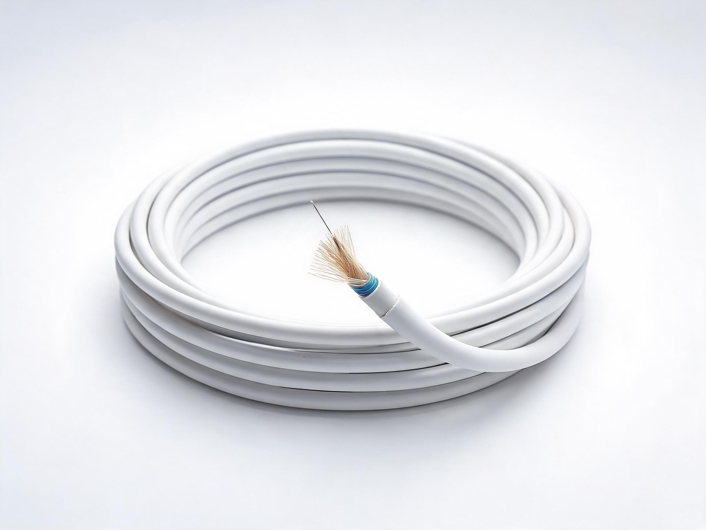
Indoor tight-buffered cable places a 900 µm buffer directly on each fiber. Fibers can be stripped and terminated individually at a panel without a splice step, which makes it the natural choice where the backbone lands directly on patch panels and ODFs. Available counts on the market commonly run from a few fibers up to 144 cores in a single jacket, in LSZH or PVC jackets with riser (OFNR) or plenum (OFNP) fire ratings matched to the zone the run passes through. The construction is also the more flexible of the two to route: a compact jacket and a bend radius typically rated at 10 × cable diameter installed (20 × under pull load) suits crowded trays and tight cabinet entries. Typical bend-radius and temperature figures should be confirmed against the datasheet of the construction ordered.
Loose-tube constructions — more common outdoors — house fibers in gel-filled tubes around a central strength member. They excel at protecting fibers over long outdoor spans (campus interconnects, carrier entries) but inside a hall they add steps at every termination point: tubes are opened, gel is cleaned, fibers are spliced to pigtails before they can land on a panel. Indoors, reserve loose tube for the segments that actually leave the building or the harsh environment.
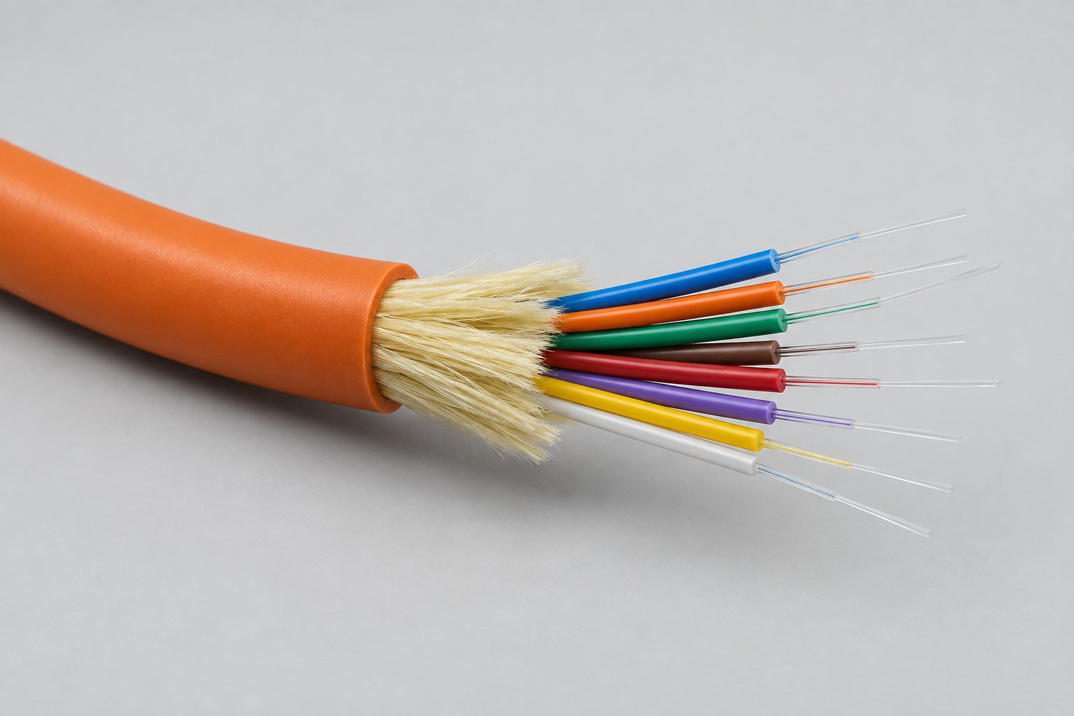
Indoor distribution cable is the middle option: a compact bundle of 2 to 48 fibers (in common indoor constructions) built for multi-core routing to a floor, a row or a data center zone, then broken out at panels. Tight-buffered distribution constructions allow direct break-out at the panel without a separate splice enclosure, which keeps riser and zone-distribution runs fast to terminate. Distribution constructions are often the practical backbone choice for row-level aggregation: one 24- or 48-core pull from the MDA to a row's HDA replaces dozens of individual runs and terminates cleanly at the row's panel.
Match the jacket rating to the zone
Data halls, corridors, risers and air-handling spaces are governed by different fire-code requirements. The most expensive jacket mistake is ordering one rating for the whole facility to simplify purchasing: a cable that passes in a general-purpose zone can fail inspection in a plenum space, and the correction is a re-pull, not a re-jacket. Match the rating to the zone — plenum (OFNP) in air-handling spaces, riser (OFNR) in vertical shafts, LSZH where low smoke and zero halogen are specified for occupied or enclosed spaces — and order each zone's run accordingly. Local code, not habit, decides.
Specify patch cords, pigtails and polarity
Patch cords look like the simplest line item in the bill of materials and are responsible for a disproportionate share of commissioning faults. Three properties decide whether they behave.
1. Optical loss per cord
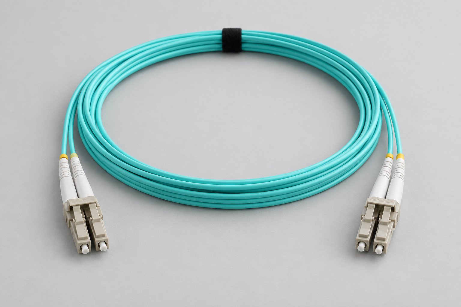
A quality factory-terminated cord is released against a per-cord insertion-loss limit, typically ≤ 0.3 dB with ≤ 0.2 dB as the typical production value, measured at the relevant wavelengths (850/1300 nm for multimode, 1310/1550 nm for single mode). Return loss is specified per polish type — typically ≥ 20 dB for multimode LC, ≥ 30 dB for multimode SC, ≥ 50 dB for UPC single mode and ≥ 60 dB for APC. These figures are typical production and release values, figures subject to datasheet. The planning-relevant point: put the per-cord limit into the purchase order and ask for test records with the goods, so incoming inspection compares measured values against the budget arithmetic done in the design, not against nothing.
2. Length discipline
Custom-length cords, made to the measured run plus a service loop of roughly 15–30 cm, eliminate the coils of slack that otherwise accumulate behind panels and in vertical managers. Excess slack is not cosmetic: coiled cord in a crowded rack bends fibers near their minimum radius, blocks airflow, and turns every future re-patch into an excavation. Ordering cords to measured lengths — 0.5 m to 30 m is a common custom range — is one of the cheapest ways to improve both airflow and loss performance.
3. Polarity in duplex channels
A duplex cord carries two fibers — transmit and receive. For the link to work, the pair must present the correct polarity at both ends, and the convention used must be consistent across the facility. A crossed pair does not degrade the signal: it removes it. The link shows no receive light at all, and the fault is invisible until the rack is dressed and powered — at which point the cord cannot be fixed in the field and must be replaced.
Polarity faults enter during manufacturing or during re-patching, and both are preventable. From manufacturing: order cords whose duplex pairs are assembled and labelled as matched transmit/receive pairs at the factory, so polarity is fixed before the goods arrive. From operations: adopt one published polarity convention (Method A, B or C in the common standards vocabulary) for the whole facility, document it at the panel level, and use labelled duplex assemblies so a rack change does not become a polarity lottery. For pre-terminated multi-fiber links, the same discipline applies at the cassette and trunk level — verify the polarity method of every pre-terminated component against the facility convention before the order, because mixing methods is a common source of cross-connect faults in MPO-based designs.
Pigtails where splices land
Where backbone fibers terminate through fusion splicing — for example, where a loose-tube campus entry lands on the MDA — pigtails move the connector termination into the factory. A factory-terminated and polished pigtail (connector on one end, bare fiber for splicing on the other) replaces the least repeatable field operation with the most repeatable one: a splice with a measurable, recorded result. Typical factory-held figures are insertion loss ≤ 0.3 dB typical / ≤ 0.5 dB max per terminated end, with return loss ≥ 50 dB UPC / ≥ 60 dB APC, figures subject to datasheet. On a 48-port panel, the rework rate difference between factory-terminated and field-terminated connectors is measured in ports reopened per panel — and each reopened port is labor that was never in the plan.
Adapters and panel density: the loss every link pays
Every mated pair in a channel passes through an adapter, so the adapter's alignment quality sets a floor under the whole facility's loss budget. A quality adapter uses a precision ceramic (zirconia) alignment sleeve to keep both ferrules on a common axis in physical contact, holding a typical insertion loss ≤ 0.2 dB and return loss ≥ 50 dB for UPC interfaces, measured at the mated pair (figures subject to datasheet).
Density multiplies the stakes. A 1U 48-port LC panel holds 48 duplex adapters — 96 mated connections in a single rack unit. Panel selection therefore deserves the same attention as cord selection: adapters whose sleeves wear unevenly under repeated patching let insertion loss creep upward and return loss fall, and a high-density panel is re-patched dozens of times during build-out and moves, adds and changes. Choosing panels built on precision sleeves, and re-checking a sample of ports after major re-patching cycles, keeps the facility's measured plant close to the values the design assumed.
Plan panel port counts with the same headroom logic as fiber counts. A panel filled to 100% at commissioning forces the first moves-and-changes wave into makeshift adapters and unlabeled ports — the exact conditions under which documentation and polarity discipline break down.
Route the pathways: bend radius, fill and labeling
Two physical rules dominate pathway quality, and both are set at planning time because they depend on tray and rack geometry, not on installer care.
Bend radius. Indoor tight-buffered and distribution constructions are typically rated at 10 × cable outer diameter when installed and 20 × under pull load (typical values, figures subject to datasheet). A 6 mm distribution cable therefore needs roughly 60 mm of installed radius — a corner in a shallow tray, a sharp cabinet entry or a zip-tie cinched too tight can all violate it. Plan the pathways so every direction change has the radius to spare: use generous tray bends, protect cabinet entries with strain-relief bushings, and train the crew to dress cables with hook-and-loop fasteners rather than tensioned ties. A fiber bent below its rated radius does not usually fail immediately — it adds attenuation that surfaces during acceptance testing or, worse, drifts upward with temperature and handling over the first months of operation.
Fill and separation. Overfilled trays make bend violations and airflow problems inevitable. Keep fiber separated from power where code requires it, leave pathway capacity for future growth (a tray filled to its limit on day one turns expansion into a shutdown), and bundle backbone fibers in sized groups so a single bundle can be pulled and dressed as one unit.
Labeling and documentation. Every permanent cable, panel port and patch cord should carry an identifier that maps to the as-built documentation. The discipline costs minutes per cable at install and saves hours per fault at 2 a.m. A data center that cannot trace a fiber from transceiver to panel has a cabling plant that only its installers understand — and they leave.
Plan the testing that will prove the plant
Acceptance testing is where the design's assumptions meet the installed reality, and it works only if the criteria were defined before the cables were ordered. Two test families cover the permanent plant:
Link loss testing with a light source and power meter measures the total insertion loss of each channel against the recorded budget for that link class (from the budget arithmetic above). Test with the method and reference cords that match the plant — single-wavelength reference methods differ, and multimode results depend on launch conditions — and record every result against the link's identifier. The pass limit for each class is the design number, not a generic threshold.
OTDR characterization on backbone spans adds the diagnostic layer: it locates splices, connectors and any anomalies along the run with distance information, producing a trace that becomes the baseline for future fault location. On multi-kilometer campus links it is essential; inside the hall it remains valuable on backbone segments because a future fault's distance reading can be matched straight to the as-built documentation.
Both test families should be specified in the installation contract with the exact wavelengths, reference method, pass limits and reporting format, so the delivered plant arrives with numbers rather than a signature. And specify the end-face inspection: the most common commissioning fault in a fiber plant is a contaminated end face, and every connector should be inspected and cleaned before it is mated — a step that costs seconds per connector and prevents the majority of marginal-loss findings.
Order from the manufacturer: the commercial terms that belong in the plan
Cabling planning ends in a bill of materials, and for most data center projects the quantities justify ordering directly from a manufacturer. Four commercial dimensions belong in the specification, because they shape both the schedule and the delivered quality.
MOQ and configuration counting
Minimum order quantities are typically quoted per configuration, not per order. A mixed order — say three cord configurations (different lengths or jacket types) — is commonly quoted at the MOQ for each configuration in the mix. Plan the bill of materials around the configurations actually needed: consolidating cord lengths and jacket types reduces the effective MOQ burden, while every extra one-off length adds a configuration. For cables, MOQ is usually quoted per construction and core count; trial quantities are often negotiable for a first order, and samples are the standard way to verify construction and termination before committing.
Lead time and schedule
Typical lead times run 7–15 working days for standard configurations, 15–25 working days for mixed or high-volume orders, counted from order confirmation (and often from deposit receipt) — figures subject to confirmation with the order. Custom fiber counts, custom lengths and printed marking extend the window. The planning consequence: order the permanent plant early, because cabling is on the installation critical path and a late reel cannot be substituted by a courier shipment. Phased backbone installations should have their cable orders sequenced against the pathway schedule, not the equipment schedule.
Customization and marking
Manufacturer-direct ordering is also where the plan's discipline gets built into the goods: custom jacket printing (circuit identifiers, zone codes), custom reel and cord lengths, customer packaging and labeling for OEM/ODM projects. Cables supplied with the project's own identifiers printed on the jacket arrive ready for the labeling scheme instead of relying entirely on on-site labels that peel and fade.
Warranty
Standard warranty across this category is 12 months from shipment date, covering manufacturing defects — construction faults, out-of-specification optical performance on the delivered goods, connector end-face defects at delivery. It does not cover installation damage, use beyond rated bend radius or tensile limits, or handling faults after delivery. Confirm the claim process and what documentation (batch references, test records) the manufacturer expects, and keep the packing labels until incoming inspection is complete, because the batch reference is what allows a claim to be traced to the production record.
Assemble the plan into a specification
The output of all the decisions above is a short, checkable specification. A complete data center cabling plan includes:
- The distribution-area map (MDA/IDA/HDA/EDA) with measured installed distances per segment.
- The topology decision and the ToR/MoR/EoR layout per row.
- Fiber grades per segment (multimode grade or single mode) with the reach figures confirmed against the specified transceivers.
- Backbone fiber counts with the demand math (active, planned, redundant, spare) shown.
- Link budget tables per link class with the assumed loss per element.
- Cable constructions per zone with jacket and fire ratings matched to local code.
- Cord, pigtail and adapter specifications with per-cord and per-pair loss limits, polarity convention and custom lengths.
- Pathway rules (bend radius, fill, labeling) and the acceptance test plan with methods, wavelengths and pass limits.
- The bill of materials with configurations consolidated, MOQ/lead-time implications noted, and warranty terms stated.
That document is short enough to review in one sitting and complete enough to hand to an installer, a procurement team and the manufacturer without follow-up clarification. Most of the expensive faults described in this guide — wrong jacket ratings, crossed polarity, marginal cords, overfilled trays, missing headroom — are absent by construction from a plan that answers these questions explicitly.
Frequently asked questions about data center fiber cabling
How far apart can the MDA and HDAs be before fiber grade becomes the deciding factor?
Multimode OM4 comfortably covers intra-hall distances: typical 10G reach is around 400–550 m and 100G SR-class reach is around 100–150 m (figures subject to the transceiver and cable datasheets). Once a segment exceeds those figures — a cross-building backbone, a separate facility on the same campus, a carrier handoff — single mode OS2 becomes the practical choice, and its attenuation (typically ≤ 0.36 dB/km at 1310 nm) makes even multi-kilometer spans routine. Measure the installed distances, compare them against the transceiver reach for the speed you are deploying, and let the comparison decide; do not guess from floor-plan distances.
Should we just build the entire facility in single mode?
It is a legitimate strategy, and an increasing number of large facilities do exactly that. Single mode removes reach as a constraint and simplifies the inventory to one fiber family, at the cost of higher transceiver prices on the many short equipment-facing links. Multimode OM4 remains cost-effective where transceiver volume is high and runs stay within reach. The decision rests on the facility's size, the upgrade horizon, and how the optics cost curve is expected to move; the safest hedge is a single-mode backbone with multimode (or SWDM-capable) horizontal, or single-mode backbone counts provisioned for future migration regardless of what today's equipment uses.
Are pre-terminated MPO trunks a better approach than field-terminated backbone cables?
Pre-terminated trunks shorten installation dramatically — a factory-assembled MPO trunk plugs in within minutes — and move quality control to the factory, which is why they dominate high-density 40G/100G builds. The trade-offs are planning discipline and polarity: trunks are ordered to exact lengths, their polarity method must match the facility convention across every cassette and trunk, and a mis-ordered trunk length means rework at the factory rather than a field trim. Field-terminated tight-buffered backbone remains the more forgiving choice where lengths are uncertain, terminations are spread over time, or the crew splices routinely. High-density rows with fixed geometry favor pre-terminated; everything else favors flexibility.
How much spare capacity is the right amount?
For backbone counts, 25–50% over projected demand is the common planning range: lower when the projection is confident and pathways are easy to extend later, higher when expansion plans are vague or pathway work is disruptive. The cost asymmetry justifies biasing high — fibers inside a cable being pulled today are cheap, and fibers that require a second installation campaign are not. The same logic applies to panel ports (plan headroom at every HDA panel) and to tray fill (never commission a tray at its limit).
What mistakes show up most often in real projects?
Five account for most of the avoidable cost: ordering one jacket rating for the whole facility and failing inspection in plenum zones; leaving polarity to chance instead of ordering factory-labelled duplex pairs and enforcing one convention; treating patch-cord loss as a commodity instead of putting per-cord limits in the purchase order; filling trays to their limit on day one so expansion becomes shutdown work; and skipping the link-budget arithmetic, so marginal components consume the reserve and links fail acceptance — or worse, fail later under load. Every one of them is preventable at the planning stage described in this guide.
Where a manufacturer fits into the plan
Most of the components in a data center cabling plan — backbone cables, distribution and tight-buffered constructions, patch cords, pigtails, adapters and panels — come from a small set of fiber optic manufacturers, and the differences between suppliers show up in the same places the design cares about: per-cord release limits actually measured and recorded, precision alignment sleeves in adapters, jacket ratings matched to order rather than approximated, custom lengths and marking that carry the project's labeling scheme into the goods, and test documentation that lets incoming inspection verify against the design numbers rather than trust them.
When requesting quotations, send the specification you assembled — segment distances, fiber grades, counts, loss limits, polarity convention, jacket ratings, marking requirements — rather than a parts list. A manufacturer who receives the design context can confirm configurations, propose consolidations that reduce configuration counts and MOQ impact, and state measured figures against your acceptance criteria. Nexora manufactures fiber optic connectivity in Shenzhen — indoor tight-buffered and distribution cables, OM3/OM4 and single-mode patch cords in custom lengths from 0.5 m to 30 m, factory-terminated pigtails for splice points, and LC/SC/FC adapters on zirconia sleeves — with quality control across 30+ QC stations, OEM/ODM support for custom marking and packaging, and a 12-month warranty from shipment date on its products.
Send us your row count, the distances between distribution areas, the transceiver types you are deploying and the counts you have projected, and our team will confirm the cable constructions, cord configurations and panel components that match the plan — with figures subject to datasheet on every optical value, so your acceptance testing compares like against like.