
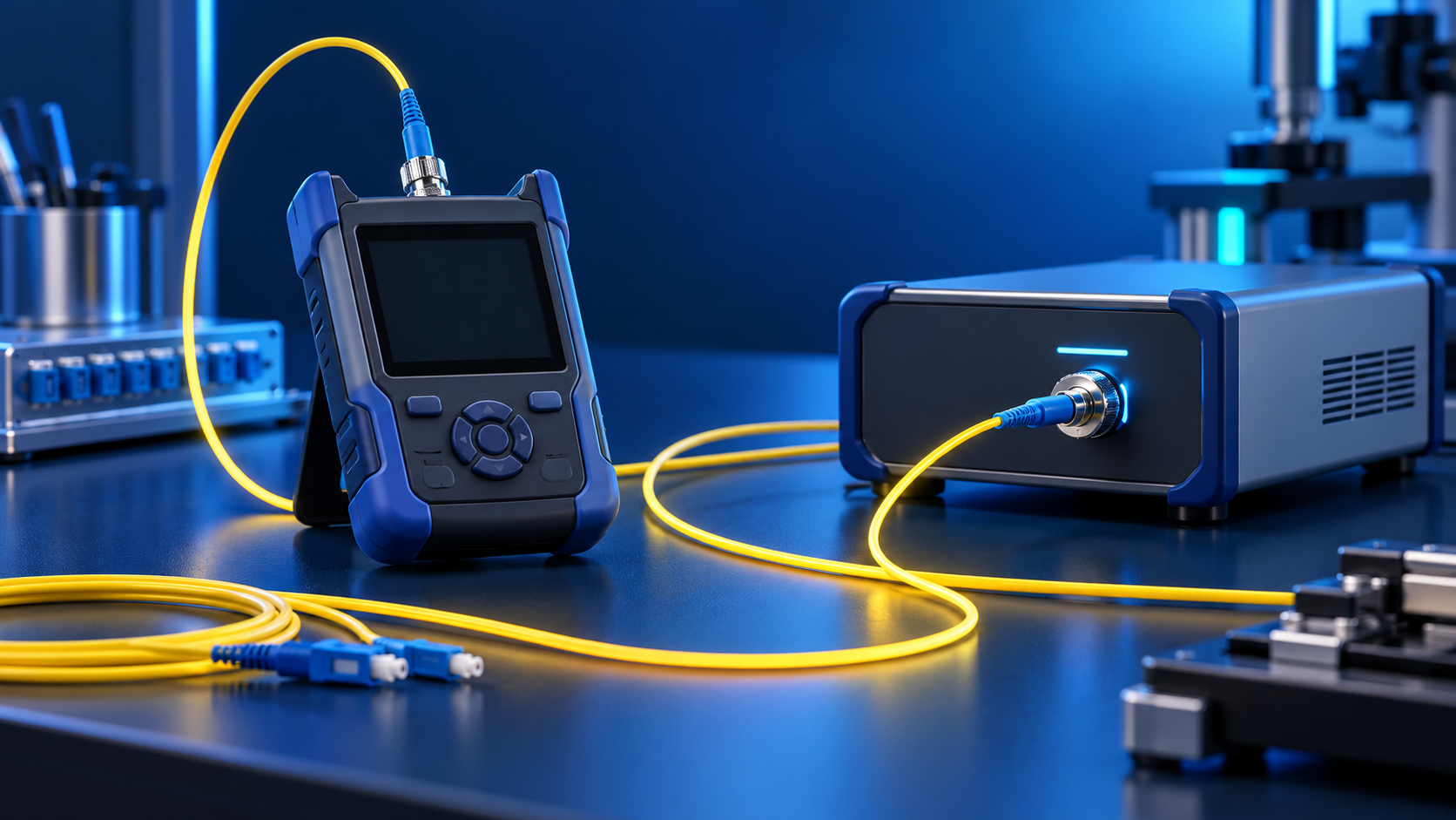
A practical B2B guide to testing a fiber optic link with a light source and power meter (OLTS): what the measurement captures, reference methods, screened test cords, loss limits at 1310/1550 nm, bidirectional testing, acceptance reporting and failed-link troubleshooting.
You finished the pull, closed the splice closures, dressed the rack, and the link lights are green. Then the acceptance test comes back with a number nobody expected: 2.8 dB of insertion loss on a route that was budgeted at 1.4 dB. The contractor says the cable is fine. The network owner says the link does not meet spec. Both can be right, and the argument usually happens because nobody agreed, before the project started, on how the link would be tested, with which reference method, which test cords and which pass limits.
That is why the light source and power meter pair — often called an OLTS, or optical loss test set — remains the reference method for link acceptance in fiber optic projects worldwide. It does not draw a trace like an OTDR and it does not localize faults like a visual fault locator. What it does is more important at handover time: it measures the total loss of the completed link, end to end, at the wavelengths the network will actually run at, and it produces a single number that can be compared directly against the loss budget you calculated when you ordered the cable.
This guide is written for the people who carry that responsibility: network engineers, integrators, contractors and the procurement teams who buy the cable, the patch cords and the test cords the whole procedure depends on. It walks through what the measurement actually captures, how the 0 dB reference is set and why the choice of reference method changes every reading on the report, which loss limits to apply at 1310 nm and 1550 nm, how to work a bidirectional test, and what to do when a link fails. Along the way it also covers the component that quietly decides whether your results are trustworthy — the reference test cords — and what to check before you order them.
Why Insertion Loss Testing Decides Whether Your Fiber Link Gets Accepted
Every optical link has a finite loss budget: the difference between what the transceiver launches and the minimum power the receiver needs to meet its error-rate specification. Fiber attenuation consumes most of that budget, and the remainder is spent on splices, connectors, splitters and margin. When a link is installed, the question is not whether light comes out the far end — it almost always does — but whether the total consumption stays inside the budget with margin to spare across the life of the network.
An insertion loss test answers exactly that question. The instrument pair injects a calibrated, stable optical signal at one end and measures how much of it arrives at the other end. The difference, expressed in decibels, is the link's insertion loss. Compare that number against the loss budget and you have a pass/fail decision that is defensible in a contractual sense: the method is standardized, the equipment is calibrated, the reference condition is documented, and the result can be reproduced by a second crew with the same limits.
For the buyer, this test is also where money changes hands. Acceptance criteria written into the contract almost always reference measured insertion loss at defined wavelengths. If the limits, reference method and test cord grades are not fixed in the specification, the same physical link can "pass" with one crew's setup and "fail" with another's — not because the fiber changed, but because the measurement conditions changed. A few decibels of disagreement at handover can cost weeks of dispute, and the most common root cause is not a bad cable: it is an under-specified test procedure.
That is the practical reason to understand this test even if you never hold the meter yourself. If you procure the cable, the patch cords and the test cords, the quality of your components determines what the crew can achieve with a correct method — and no method can rescue a link assembled from cords with unknown insertion loss or mismatched polish types.
What a Light Source and Power Meter Test Actually Measures
The principle is simple enough to explain in one sentence: you launch a known optical power into the link and measure how much arrives. The execution is what makes the difference between a number you can defend and a number that gets challenged.
A stable light source emits continuous-wave power at one or more selected wavelengths — for single-mode networks typically 1310 nm and 1550 nm — with output power held constant within a tight tolerance over the test period. An optical power meter at the far end converts arriving light into a reading in dBm, and in relative mode expresses the difference against the stored reference level in dB. The pair, used with correctly selected reference cords, measures the total attenuation of everything between them: the fiber, the fusion splices, the mechanical splices, the connectors at both ends, and every mated adapter in between.
Three properties make this measurement the acceptance standard rather than a rough field check. First, it is total-loss measurement: the meter sees the sum of all contributors, which is exactly what the transceiver at each end will experience. Second, it is wavelength-specific: measuring at 1310 nm and 1550 nm reproduces the conditions the actual transmission equipment will see, rather than approximating them at an arbitrary wavelength. Third, it is reference-relative: the 0 dB point is set on the bench before testing begins, so the reading reflects only the link under test, not the instruments or the cords used to connect them.
What the test deliberately does not do is locate anything. A failed reading tells you the link is lossy; it does not tell you where. Localization is the job of an OTDR trace or a visual fault locator, and a disciplined acceptance workflow uses all three tools in sequence: OLTS to verify the pass/fail number, OTDR to characterize and document the route, and a VFL for quick continuity and fault finding when something needs to be fixed. Understanding which instrument answers which question prevents the most common field argument — crews presenting an OTDR trace as evidence against an OLTS result, when the two instruments measure different things under different conditions.
OLTS vs OTDR vs VFL: Which Tool Answers Which Question
The three instruments are complements, not substitutes. The table below summarizes what each one measures, what it is used for in a project lifecycle, and where its blind spots are.
| Instrument | What it measures | Primary use | Key limitation |
|---|---|---|---|
| Light source + power meter (OLTS) | Total end-to-end insertion loss at selected wavelengths | Acceptance testing against a loss budget; link certification | No distance information; cannot localize a fault |
| OTDR | Backscatter profile along the fiber; event locations and individual event losses | Route documentation, fault localization, splice and connector characterization | Dead zones hide near-end events; loss figures are estimates, not the transceiver's experience |
| Visual fault locator (VFL) | Visible red light leakage at breaks, bad bends and connector defects | Quick continuity checks, finding macro-bends and broken fibers over short runs | Short range; cannot measure loss; not usable on armored or jacketed routes beyond a few hundred meters |
A practical acceptance routine on a new build looks like this in sequence: visually inspect and clean every connector end face before it is mated; run the OLTS bidirectional test at the contract wavelengths; run an OTDR bidirectional trace to document the route and record event positions; and keep the VFL on the truck for the exceptions. The OLTS result is the contractual number; the OTDR trace is the diagnostic map; the VFL is the quick sanity check. When a dispute arises, the resolution almost always comes from comparing the OLTS result against the loss budget calculation, then using the OTDR to explain any excess.
If your project specification references an OTDR acceptance procedure only, it is worth adding an OLTS clause: the two documents answer different questions, and OTDR event losses do not add up to the true end-to-end loss a transceiver sees. Conversely, an OLTS-only specification leaves you without a map when a link fails — so most well-written specs require both.
The Test Kit: What You Actually Need on Site
A complete insertion loss test kit is more than the two instruments. Missing or low-grade accessories are the most common reason a crew produces readings that cannot be reproduced, so it is worth listing the full inventory before mobilizing:
- Stable light source. Emits calibrated continuous-wave power at 1310 nm and 1550 nm for single-mode work (plus 850 nm and 1300 nm for multimode). Output stability over the test session matters more than absolute output power; a source that drifts between setting the reference and testing the link corrupts every reading after it.
- Optical power meter. Measures arriving power in dBm and, critically for this workflow, stores a relative 0 dB reference. Detector type and calibration wavelength range should match the fibers being tested.
- Reference test cords. Three or more high-grade patch cords matching the connectors and polish of the link under test. These are measurement instruments, not accessories — their grade caps the accuracy of the entire session.
- Adapters (mating adapters). One per cord-to-cord junction in the reference setup and the test setup, matched to the connector family and polish. A worn or contaminated adapter adds its own uncontrolled loss.
- One-click cleaners and lint-free wipes. Every end face is cleaned before every mate. This single habit eliminates the most frequent cause of false failures.
- Fiber inspection scope (video microscope). To verify end faces before mating. Inspection before cleaning and after cleaning is the sequence specified in industry practice: inspect, clean if needed, inspect again, then connect.
- Test record template. A fixed form for link ID, wavelength, reference method, crew, instruments and serial numbers, measured loss per direction, and margin. More on this in the reporting section.
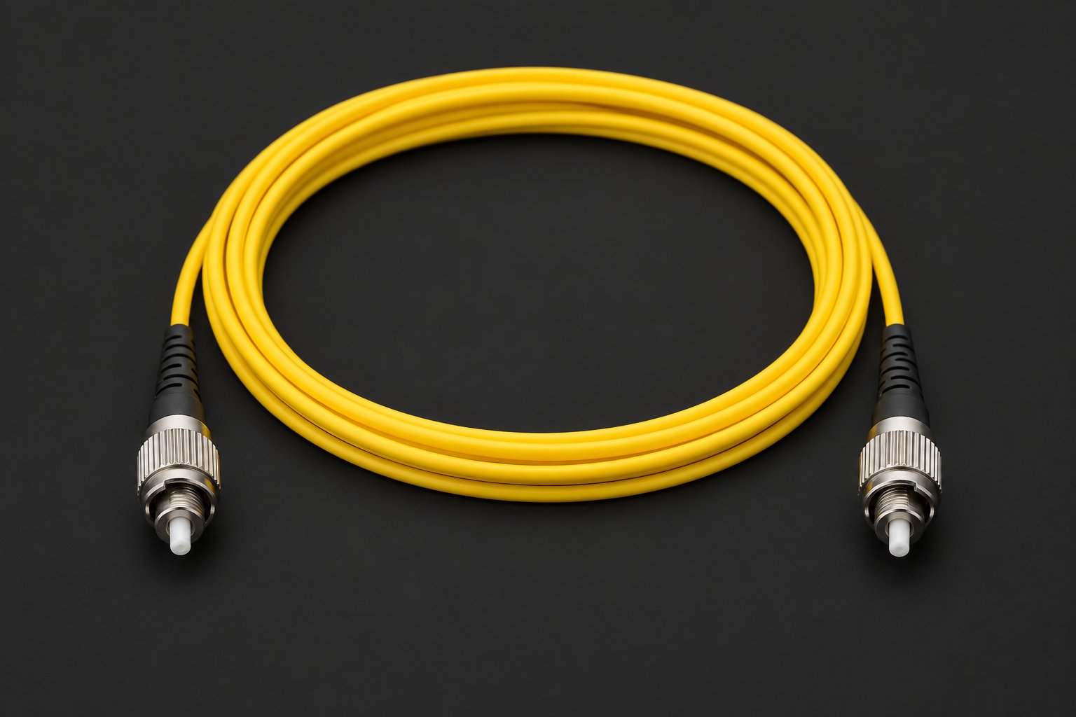
The instrument choice also deserves a comment on connectors. On a test bench where cords are mated and unmated all day, threaded connectors such as FC hold their position and their reading in a way that spring-latched connectors on an over-worked adapter may not — which is why many test labs keep FC-terminated reference cords for bench verification even when the field links use LC or SC. The image above shows the threaded coupling nut that keeps the ferrule seated through repeated mate cycles; if your crew verifies instrument calibration between site visits, this is the cord style that survives that duty.
Reference Test Cords: The Component Most Buyers Under-Specify
Every insertion loss reading passes through the reference cords. Whatever excess loss or reflection they contribute is either added to or subtracted from the link under test, depending on the reference method, and no field procedure can compensate for a bad cord. Treating reference cords as consumables rather than as measurement standards is the single most expensive shortcut in link testing.
What separates a test-grade cord from an ordinary patch cord is not a different connector family but the discipline around its manufacture and screening. A test-grade single-mode cord is built on a standard fiber such as ITU-T G.652D, terminated with connectors whose end faces are inspected against the acceptance criteria for the polish type, and screened for insertion loss and return loss at the working wavelengths — typically at 1310 nm and 1550 nm for single mode. The image below shows a typical single-mode test-grade assembly: an SC-SC construction on G.652D fiber, the workhorse configuration for access and backbone test sets.
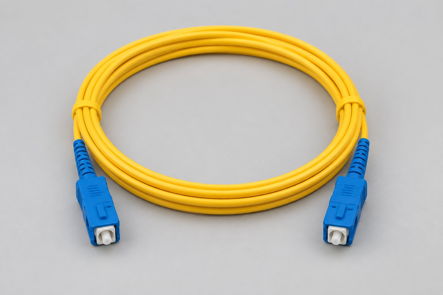
When you order test cords, the specification should cover the same fields you would apply to any patch cord order, plus the measurement context:
- Fiber type. Match the link under test: G.652D for standard single-mode routes. If a route uses bend-insensitive fiber such as G.657A1 or A2, the reference cords should match or the fiber-type mismatch contributes a small but real difference at tight bend radii; for typical panel-to-panel testing on G.652D routes, G.652D cords are the correct match.
- Connector and polish on both ends. Match the equipment and the link: SC, LC or FC, UPC or APC. Mixing polishes on a single-mode link is not a field repair — an APC port mated with a UPC cord creates a small air gap at the core that raises loss and collapses return loss, so the cord must be ordered to match the ports it will serve.
- Screened insertion loss. Test-grade cords are typically screened to an upper limit of 0.5 dB per cord with 0.3 dB typical across production, measured at 1310/1550 nm — figures per datasheet; confirm the screening limits and test wavelengths with the supplier before ordering. For loss-budget verification on tight routes, ask whether tighter screening is available.
- Return loss. UPC end faces are typically specified at 50 dB or better and APC end faces at 60 dB or better, so the reference junction does not contaminate reflectance-sensitive measurements.
- Length and jacket. Short cords (typically 1-3 m) minimize the cord's own attenuation in the reference; jacket per the environment, with LSZH for ventilated indoor spaces and PVC for general-purpose indoor use.
- Certification of the cords themselves. Ask for the per-cord test record listing measured insertion loss and return loss. A reference cord without a measurement record is an ordinary patch cord with a higher price.
Commercial terms follow the same logic as production cords. Reference-grade assemblies are custom-terminated, so typical minimum order quantities start at 100 pieces per configuration, with standard configurations shipping in 7-15 working days and mixed or high-volume orders in 15-25 working days — terms counted from order confirmation and deposit receipt, and confirmed on the quotation. Warranty for the cords themselves is 12 months from shipment date covering manufacturing defects; damage from field handling is excluded, which is one more reason crews treat reference cords gently, keep dust caps on, and retire any cord that has been dropped or mated dirty.
Setting the 0 dB Reference: One-, Two-, and Three-Cable Methods
Before any link is tested, the instrument pair is "zeroed": the source is connected to the meter through the reference cords and adapters only, and the meter's reading is stored as 0 dB. Everything the meter later sees is measured relative to that condition. The way this reference is built determines what the subsequent readings include — and it is the most misunderstood part of the whole procedure.
Industry practice recognizes three reference methods, commonly called the one-cable, two-cable and three-cable reference. The names count the cords between source and meter when the reference is set.
| Method | Reference setup | What the link reading includes | Typical use |
|---|---|---|---|
| One-cable reference | Source → launch cord → meter (one mated connection at the meter) | Both link-end connectors, all splices, the fiber — but excludes one connector's loss from the zero point, so readings are lowest | Maximum accuracy needs; requires a meter port matching the link connector |
| Two-cable reference | Source → launch cord → adapter → receive cord → meter (one cord-to-cord adapter) | Both link-end connectors plus one adapter loss | The most common field method; balances accuracy and practicality |
| Three-cable reference | Source → cord → adapter → cord → adapter → cord → meter (two adapters) | Both link-end connectors plus two adapter losses | Required when connectors on the link and the instrument ports differ, e.g. testing APC links with UPC-metered instruments |
Two consequences follow, and both should be written into the project test plan. First, the same physical link will yield different measured losses under different reference methods — a two-cable reference produces a reading roughly one connector-pair loss higher than a one-cable reference, and a three-cable method higher still. Comparing a crew's results against the contract limits is only meaningful when everyone used the same method. Second, the three-cable method is the standard way to handle polish or connector mismatches between instruments and link: testing an APC-terminated route with instruments that present UPC interface ports, for example, requires the reference to be set through an APC-to-APC cord chain so that the meter never mates across a polish boundary during the reference.
Whatever method is chosen, the reference is verified — not assumed — at least once per session: after setting 0 dB, remate the reference chain and confirm the meter reads within a small residual (commonly expected within about 0.1 dB for a clean, high-grade chain). If the residual is worse, the chain has a dirty end face, a worn adapter or a damaged cord, and the session must not begin until it is resolved.
Step-by-Step: Testing a Single-Mode Link in the Field
With the kit assembled and the reference method fixed in the test plan, a disciplined single-mode acceptance test follows the same sequence every time. The order matters: each step either protects the validity of the reference or eliminates a variable that would otherwise surface later as a dispute.
- Plan and label. Assign a link ID to every fiber path (for example, "ODF-A 04 → Building B IDF 12"), record the route length and the fiber type, and note the contract wavelengths and limits. Test without a naming convention cannot be audited later.
- Inspect and clean every end face. Inspect the link connectors and the reference cords with the scope; clean with a one-click cleaner; inspect again. A visible contamination ring on the scope predicts the reading before the meter is even connected.
- Set the reference. Mate the reference chain per the chosen method (two-cable is the common field default), let the source warm up per its manual — typically a few minutes — then store 0 dB on the meter at each test wavelength. Record the reference method on the sheet.
- Verify the reference. Remate the chain and confirm the residual reading is within the session tolerance (about 0.1 dB with a clean, high-grade chain). If not, clean and re-inspect until it passes; do not proceed on a drifting reference.
- Connect the link. Replace the receive cord with the link under test, keeping the launch cord in place. The connector now mating to the launch cord must be clean and inspected; this is the connector whose loss the reading will include or exclude depending on the reference method.
- Measure at each wavelength. Read and record the loss at 1310 nm, then switch the source to 1550 nm and repeat (or use a dual-wavelength source and record both). Note the reading, the link ID, the direction, the crew and the instruments.
- Reverse and repeat. Swap source and meter to test the opposite direction, or use a bidirectional-capable set. Record the second direction separately; the reporting section explains why.
- Compare and disposition. For each link and wavelength, compare the measured loss against the pass limit from the loss budget. Record pass/fail and the margin. Any failure goes into the troubleshooting sequence — not into re-testing until it passes.
Two habits distinguish professional crews from statistical ones. First, they never touch an end face after the final inspection: connector boots are held, not jackets, and dust caps go back on immediately if a cord is disconnected. Second, they record the instrument serial numbers and reference cords used per session, which is what makes a challenged result reproducible weeks later with the same chain.
Test Wavelengths and Loss Limits: What Figures to Apply
The test is only as meaningful as the limits it is compared against, and the limits come from two sources that must be kept separate: the fiber's intrinsic attenuation and the loss allowances for splices and connectors.
For standard single-mode G.652D cable, datasheet attenuation is typically ≤0.36 dB/km at 1310 nm and ≤0.22 dB/km at 1550 nm (figures per datasheet; confirm the values on the specification sheet issued with your order). A 12 km route therefore consumes roughly 4.3 dB at 1310 nm and about 2.6 dB at 1550 nm in fiber attenuation alone — before any splice or connector is counted.
Splice and connector allowances are design values, not measurement predictions. Industry practice for cabling standards such as TIA-568 and ISO/IEC 11801 allocates a typical allowance of 0.3 dB per mated connector pair and 0.1-0.3 dB per fusion splice (typical design allowances; project specifications govern). A route with two connector pairs and eight fusion splices therefore carries roughly 0.6-1.0 dB of design allowance beyond the fiber itself, plus spares and margin per the project's own rules.
The pass limit for a given link is the sum: fiber attenuation at the route length, plus splice and connector allowances, plus any project-specific margin. Writing that calculation into the test plan — before installation begins — is what turns the acceptance test from an argument into arithmetic. Our article on calculating a fiber optic link loss budget walks through the full method; the testing step in this article is simply the measurement that closes the loop against that budget.
Worked Example: Building the Expected Loss for a 12 km Route
Consider a concrete case that mirrors a common access or metro build: a 12 km underground route between two sites, built with 24-core outdoor G.652D loose-tube cable in duct, with eight fusion splices (four at joint locations in both directions of counting) and one mated connector pair at each end terminating onto patch panels.
The expected loss at 1310 nm builds up as follows: 12 km × 0.36 dB/km = 4.32 dB of fiber attenuation; 8 fusion splices × 0.1 dB = 0.8 dB; 2 connector pairs × 0.3 dB = 0.6 dB, using the typical allowances above. The total expected loss is about 5.7 dB, and a project would typically add its own margin rule — for example 1 dB — to arrive at a pass limit near 6.7 dB at 1310 nm. At 1550 nm the same route calculates to about 2.64 + 0.8 + 0.6 = 4.0 dB before margin. Figures per datasheet and typical allowances; the project specification governs.
On acceptance day, a measured 5.9 dB at 1310 nm in one direction passes with margin; a measured 8.4 dB fails by more than a decibel and a half. The number alone does not say why — that is the troubleshooting sequence later in this article — but the budget calculation has already told everyone which links deserve scrutiny and how much re-work a marginal result justifies before handover.
This is also the moment the cable grade pays for itself. Cable supplied with per-reel attenuation test records lets the crew compare measured link loss against the factory's reel data instead of a datasheet maximum, which shortens the diagnostic path when a result is marginal. When ordering cable for routes that will be acceptance-tested this way, ask for the per-reel test report and keep it with the project file.
Bidirectional Testing: Why One Direction Is Not Enough
A single-direction insertion loss reading hides a systematic effect: the loss of a mated pair depends on which side receives. When two connectors with slightly different mode field diameters or core alignment mate, the junction loses more light in the direction that launches from the smaller effective core into the larger one than in the reverse direction. The same junction can therefore measure, for example, 0.35 dB one way and 0.15 dB the other — both readings are real, and the link's true behavior is the average of the two.
Bidirectional testing resolves this in the way acceptance standards intend: measure the link from end A to end B, then swap the instruments and measure B to A, and report the average per link and wavelength. On long routes with many splices, the direction effect compounds — a route with a dozen moderately misaligned splices can show a decibel of asymmetry — so bidirectional averaging is not optional on anything beyond short campus runs.
Operationally, the swap is where errors creep in. The crew must swap the cords at the instruments, not remate the link mid-test, and the reference must not be reset between directions with a different chain. Crews that plan the swap — cord tags on each instrument, a fixed sheet layout with two direction columns per link — complete the second direction in minutes and produce reports that survive audit.
Multimode Links: What Changes with OM3, OM4, and OM5
The same instrument pair tests multimode links, but three variables change. The wavelengths move to 850 nm and 1300 nm. The source type matters: VCSEL-based sources at 850 nm approximate the transceivers used on 10G-and-above links, while older LED sources overfill the fiber and measure a different loss than the equipment will experience; for modern graded-index fiber, controlled launch conditions (encircled flux) are the accepted way to make readings comparable between crews and consistent with the equipment's launch. And the loss limits are much smaller per meter — multimode attenuation is typically around 3.0-3.5 dB/km at 850 nm — which makes connector and adapter quality a proportionally larger share of the budget.
Reference cords for multimode work must match the fiber category: OM3, OM4 or OM5 cords for the corresponding links, since overfilled launch conditions differ between 50 µm categories. Mixing an OM3 reference cord into an OM4 link test adds a launch-condition error that shows up as optimistic or pessimistic readings depending on the direction — the same argument as mode field mismatch in single mode, with different physics.
If your project mixes multimode backbone (typical inside buildings and data centers) with single-mode campus runs, write the test plan in two parts: one for each fiber type, each with its own wavelengths, source type, reference cords and limits. Attempting to run one procedure across both types is a common source of invalid comparisons on mixed campuses; for guidance on choosing between the multimode grades themselves, see our comparison of OM3, OM4 and OM5 fiber.
Recording Results and Building an Acceptance Report
The test is not finished when the meter shows a number; it is finished when the result is documented well enough that another engineer can reproduce it. A defensible acceptance report for each link records, at minimum:
- Link ID, route description, fiber type and route length
- Test wavelengths, reference method, and the instruments and reference cord serial numbers used
- Measured insertion loss per direction and per wavelength, and the bidirectional average where applicable
- The pass limit applied (with the specification version) and the resulting margin
- OTDR trace file references for the same links, so any marginal result has a diagnostic map attached
- Crew, date, and environmental notes for outdoor work (temperature matters on routes near their operating limits)
Modern test sets export this automatically; what they cannot supply is the discipline around it. Two fields are the ones auditors and network owners check first: the reference method recorded per session, and the pass limit version applied. Reports missing those two fields are the ones that reopen disputes months later.
For the buyer, the report is also a supplier-quality document. If certain links consistently sit close to the limit, the pattern often points back to component quality — connector end faces, adapter wear, or cord grade — rather than workmanship. Keeping the per-link numbers in one file across the project makes those patterns visible, which is exactly the evidence you want when deciding whether a component supplier change is justified on the next phase.
When the Link Fails: A Structured Troubleshooting Sequence
A failed insertion loss reading triggers a sequence, not a scramble. The order below resolves the majority of excess-loss findings without disturbing good work:
- Re-verify the reference chain. Before touching the link, remate the reference cords and confirm the 0 dB residual is still within tolerance. A drifted reference invalidates every reading in the session, so this check costs two minutes and can save a day.
- Re-clean and re-inspect the link connectors. Contamination at either panel is the most frequent cause of a marginal failure. Clean, inspect, remate, and re-measure the link. A large share of "failed" links pass at this step.
- Check for tight bends and crush points. Excess loss that survives cleaning often lives at a bend: a cable dressed too tightly at a panel entry, pinched under a rack leg, or kinked in a duct. A visual fault locator shows macro-bend leakage as red glow through the jacket on short runs and is the fastest way to find them; for anything longer, an OTDR trace locates the event by distance.
- Run an OTDR trace on the failed link. The trace turns "8.4 dB total" into a map: which splice is lossy, whether a connector is dirty or damaged, and whether a section shows the gradual attenuation climb that suggests water ingress or crushing. If you are building the acceptance workflow, our guide to using an OTDR for new-installation acceptance covers the trace settings and event interpretation.
- Isolate by substitution. Replace the reference cords with known-good spares and re-measure; if the number moves, the cords were the problem. Patch in a known-good factory-terminated cord at one end to separate panel connector loss from route loss.
- Escalate with evidence. If the route itself is the cause, the OTDR trace and the re-test history are what the cable or splice contractor needs. A structured sequence produces that evidence naturally; a scramble produces opinions.
The same sequence, minus the instruments, is worth training every field crew on — including the habit of cleaning before every mate, not only after a failure. Our article on cleaning and inspecting fiber optic connectors covers the inspection grades and cleaning tools in detail, and the visual fault locator guide covers the quick diagnosis tricks for short links.
Common Sourcing Mistakes with Test Cords and Kits
Procurement sits upstream of all of this, and a recurring pattern of ordering mistakes shows up across projects. Each one is cheap to prevent at purchase-order stage and expensive to discover on site:
- Ordering unscreened cords as reference cords. Without per-cord insertion loss and return loss records, there is no way to know whether the cord chain can set a valid reference. Specify screening limits (for example, 0.5 dB max per cord with 0.3 dB typical, figures per datasheet) and require the test record with the shipment.
- Leaving the polish unspecified. "SC-SC single mode" is not a complete specification; UPC and APC are different end faces and are not interchangeable. Every mixed-polish incident at handover traces back to an order that did not state the polish on both ends. Our guide to reading patch cord specs explains how insertion loss, return loss and polish types appear on a datasheet.
- Buying the cheapest possible patch cords for the test bench. Bench cords take thousands of mate cycles. Threaded FC cords hold their connection through that duty; overworked latched connectors and worn adapters silently degrade reference quality long before anyone notices.
- Mismatching fiber categories. G.652D cords for G.652D routes; OM3/OM4/OM5 cords matched to the multimode grade; G.657 cords where routes use bend-insensitive fiber. The mismatch is usually small, which is exactly why it goes unnoticed until results are compared across crews.
- Under-ordering quantities. A two-cable reference needs three cords minimum per set, and duplex testing doubles that. Crews that run short start reusing unverified cords — and the reference quality is gone.
- Ignoring the jacket and length requirements. Reference cords live in cases and panels: 1-3 m and LSZH or PVC per the environment. Six-meter cords coil into panels, add attenuation, and invite bends.
For a broader view of how cord grades, adapters and polish choices fit together when specifying connectivity for a project, our buyer's guide to fiber optic patch cords and adapters covers the selection logic in one place.
How Nexora Supports Test-Cord Supply and Custom Configurations
Nexora manufactures fiber optic connectivity and cabling products in Shenzhen, and reference-grade patch cords are a routine part of that production rather than a special case. The same SC-SC single mode G.652D cord used for access and panel links is available as a test-grade assembly, and the factory release process is built around the figures an acceptance test depends on: every cord passes connector end-face inspection, insertion loss measurement and return loss measurement before packing, with insertion loss screened to ≤0.5 dB max per cord and ≤0.3 dB typical across production at 1310/1550 nm, and return loss of ≥50 dB for UPC and ≥60 dB for APC end faces — figures per datasheet, confirmed on the specification sheet issued with your order.
For crews that standardize on threaded connectors for bench verification, the FC-FC single mode patch cord carries the same screening discipline with a threaded coupling nut that holds its position through repeated mate cycles. Both families are available in custom lengths from 0.5 m to 30 m (SC-SC as simplex or duplex; FC as simplex), with LSZH or PVC jackets, and with UPC or APC end faces built to match the ports they will serve. Where a project needs a tighter screening limit for loss-budget verification, that requirement can be stated at quotation stage and confirmed against the production process.
Ordering terms follow the factory's standard practice: minimum order quantities of 100 pieces per configuration for patch cords, lead times of 7-15 working days for standard configurations and 15-25 working days for mixed or high-volume orders, counted from order confirmation and deposit receipt. Test records listing measured insertion loss and return loss can be supplied with the order — per cord or as a batch summary — and OEM/ODM labeling and packing are available for teams that issue cords as standard kits to their crews. Products are covered by a 12-month warranty from shipment date against manufacturing defects.
On the cable side, the same facility produces the outdoor G.652D loose-tube cable that acceptance tests ultimately measure, in 2-288 core counts for backbone, metro and access routes, with per-reel attenuation test records available on request. The manufacturing base behind both product families — a 16,000+ m² facility with 12 production lines, 180+ employees, 30+ QC stations, and 500+ OEM/ODM projects delivered to customers in 50+ countries — is what makes a consistent, screened cord supply practical at project quantities rather than only at laboratory volumes.
Frequently Asked Questions
What is the difference between an insertion loss test and an OTDR test?
An insertion loss test (OLTS) measures the total end-to-end loss the transceiver will experience; an OTDR measures backscatter along the fiber to locate and characterize individual events. The OLTS result is the acceptance number; the OTDR trace is the diagnostic map. They answer different questions and are used together, not interchangeably.
Which reference method should our project use?
The two-cable reference is the most common field default because it balances accuracy and practicality. Use the three-cable method when the link connectors or polish differ from the instrument ports, and reserve the one-cable method for cases where maximum accuracy is required and the meter port matches the link connector. The critical rule is consistency: everyone on the project uses the method written in the test plan.
What loss limits should we apply at 1310 nm and 1550 nm?
Build the limit from the loss budget: fiber attenuation at the route length (for G.652D, typically ≤0.36 dB/km at 1310 nm and ≤0.22 dB/km at 1550 nm, figures per datasheet), plus typical design allowances of about 0.3 dB per connector pair and 0.1-0.3 dB per fusion splice, plus the project's own margin. The project specification governs; record which version was applied.
Can we test an APC link with a UPC-terminated test set?
Yes, using the three-cable reference method: the reference is set through a cord chain that mates APC to APC, so the meter never mates across a polish boundary. The link connectors are then tested through matching APC cords. What you cannot do is mate a UPC cord directly into an APC port — the air gap at the core adds loss and collapses return loss.
Why do our two crews get different numbers on the same link?
Almost always one of three causes: different reference methods, dirty or unscreened reference cords, or a single-direction reading compared against another crew's bidirectional average. Fix the test plan, standardize on screened reference cords with records, and require bidirectional averaging, and the crews will converge.
How often should reference test cords be replaced?
Treat them as measurement standards: retire any cord that has been dropped, mated dirty, or shows a visible end-face defect under the scope, and verify the chain's 0 dB residual at the start of every session. Keeping two verified spare sets per kit means a suspect cord never becomes a reason to keep testing.
What should we ask a supplier for when ordering test cords?
Fiber type matched to the route, connector family and polish on both ends, screened insertion loss and return loss limits with per-cord test records, length and jacket, simplex or duplex, and the commercial terms (MOQ per configuration, lead time from order confirmation and deposit receipt, warranty of 12 months from shipment date). A supplier who can state all of these is supplying a measurement tool; one who cannot is supplying a patch cord.
Do we still need an OTDR if the OLTS passes?
Most acceptance specifications require both: the OLTS proves the loss number, and the OTDR documents the route so that future faults can be located against a baseline. A link that passes today with no trace on file is harder and slower to diagnose when it degrades in three years.
Conclusion: Fix the Method Before You Need the Number
An insertion loss test is simple to run and easy to invalidate. The instruments matter, but the reference method, the grade of the reference cords, and the cleanliness discipline decide whether the number on the report can be defended at handover. The procurement lesson is just as direct: screened test cords with per-cord records, polish stated on both ends, fiber categories matched to the routes, and a supplier who publishes the screening figures are all cheaper than a single disputed acceptance test.
If you are planning an upcoming project, the sequence that works is: write the test plan (wavelengths, reference method, limits) alongside the loss budget; order the cable and the screened reference cords together; and train the crew on the inspect-clean-connect habit before mobilization. When you are ready to specify the components, the guides below cover the decisions this article assumed:
- How Do You Calculate a Fiber Optic Link Loss Budget for Your Network Design? — the budget the test is measured against
- How Do You Read Fiber Optic Patch Cord Specs? — insertion loss, return loss and polish types on a datasheet
- Which Fiber Optic Cable Should You Order: G.657 or G.652D? — matching fiber type to the route
- OM3 vs OM4 vs OM5 Multimode Fiber — specifying multimode grades for indoor and data center links
- How Do You Clean and Inspect Fiber Optic Connectors? — the inspect-clean-connect habit
And when it is time to order the cords the whole procedure depends on, start from the SC-SC single mode G.652D patch cord or the threaded FC-FC single mode patch cord, both available with UPC or APC end faces, custom lengths and per-cord test records — or browse the outdoor G.652D single mode fiber optic cable the acceptance test ultimately measures. Tell us the fiber type, the polish on both ends and the screening limits your test plan requires, and we will confirm the configuration and supply the test records with the shipment.