
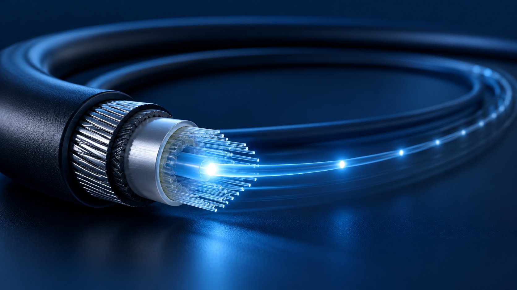
A buyer's guide to calculating the fiber optic link loss budget: which loss components belong in it, typical attenuation values for single mode and multimode links, step-by-step calculation with worked examples, return loss and polish type considerations, and how to verify the finished link with OLTS and OTDR testing.
Every fiber optic link, no matter how simple it looks on a drawing, is a chain of individual loss events: kilometers of glass that attenuate light, connectors that mate two polished end faces, splices that fuse two fibers together, and occasionally splitters or patch panels that add their own contribution. When a network is designed, all of these events are added up into a single number — the optical link loss budget — and that number decides, before a single cable is pulled, whether the transceivers at both ends will see enough optical power to communicate reliably.
For B2B buyers the calculation matters in three very practical ways. First, it tells you whether the cable construction, fiber count, and connector plan you are about to order can actually support the transmission distance and data rate your project assumes. Second, it gives you an acceptance criterion: when the installer hands over test results, you compare measured loss against the calculated budget instead of accepting vague assurances that "the link works." Third, it protects you from the two classic failure modes of cabling projects — links that are over-designed and waste money, and links that quietly fail margin tests because nobody added up the connector losses before ordering.
This guide explains, in buyer's terms, what a fiber optic link loss budget is, which components belong in it, how the numbers change between single mode G.652D, G.657, and multimode OM3/OM4 links, how to calculate a budget step by step with worked examples, and how to verify the result after installation. Wherever a figure is quoted as a typical industry value, treat it as a reference point for planning — the datasheet of the specific cable, patch cord, or transceiver you purchase always governs, and your acceptance test is what confirms the finished link.
What Is a Fiber Optic Link Loss Budget and Why Does It Decide Whether Your Network Works?
A link loss budget is the total amount of optical power that can be lost between a transmitter and a receiver while the link still operates within specification. Every active optical transceiver — a 10G SFP+ module, a 25G SFP28, a 40G QSFP+ SR4, a GPON OLT and ONU — is characterized by two numbers that define this window: the transmit power the module launches into the fiber, and the receiver sensitivity, which is the minimum power the module needs to recover the signal at a defined bit error rate.
The difference between what the transmitter launches and what the receiver needs is sometimes called the available power budget. A link works when the sum of all losses along the path — plus a safety margin — is smaller than that available power. Written as a simple inequality:
Transmit power − Receiver sensitivity ≥ Total link loss + Safety margin
Consider a typical 10G single mode transceiver pair. Transmit power is often around 0 dBm and receiver sensitivity around −14 dBm for a short-reach module, which gives an available power budget of roughly 14 dB. If your cable plant accumulates 11 dB of loss, the link closes with about 3 dB of margin — healthy. If the same plant is built with 13.5 dB of loss, the link may pass on installation day and then drift out of specification over the years as connectors age, splices degrade, or a patch cord is replaced with a lower-grade one. That is why designers add a safety margin, commonly 1 to 3 dB, on top of the calculated component losses: the margin absorbs aging, repair splices, and the small measurement uncertainties of field testing.
The loss budget also frames a commercial question buyers should ask consciously: what am I paying for in the cable plant? Attenuation in the cable itself is priced per kilometer of glass quality and cable design. Connector loss is priced in the precision of ferrule polishing and the quality of adapters. Splice loss is priced in labor skill and splicing equipment. When you understand which components consume the budget, you can decide where spending more genuinely buys reliability — and where a standard construction is perfectly adequate.
There is a second, often overlooked dimension: return loss. While insertion loss measures how much light fails to reach the receiver, return loss measures how much light is reflected back toward the transmitter. Laser sources used at 10G and above are sensitive to reflections, which destabilize the laser and raise bit errors. A link can meet its insertion loss budget and still misbehave because one connector was mated with the wrong polish type. Buyers who specify both insertion loss and return loss — and test both at acceptance — avoid the most common "specification passed, network unstable" scenario. The two are specified and verified together on quality patch cords, which is why the topic reappears later in this guide.
Which Loss Components Belong in Your Fiber Optic Link Loss Budget?
A complete loss budget adds up five families of components. Missing one of them is the most common reason calculated budgets turn out to be optimistic.
Cable attenuation
This is the distributed loss of the fiber itself, expressed in dB per kilometer and multiplied by the actual route length of the cable — not the geographic distance between the two sites. Cables rarely follow the shortest path: they follow ducts, trays, risers, and trenches, and route length is commonly 20 to 50 percent longer than the straight-line distance. Use the route length shown on the cable schedule, or add a conservative routing factor when the exact route is not yet fixed.
Connector pairs
Every mated connector pair — at a patch panel, an ODF, an equipment port, or a wall outlet — consumes budget. In loss calculations, connectors are counted in mated pairs: a patch cord plugged into a panel connector at each end creates two mated pairs, not four connector "halves." Field-terminable connectors, mechanical splices, and pre-polished splice-on connectors each have their own loss characteristics, and their datasheet values should be used rather than a generic number.
Splices
Fusion splices connect cable sections and repair breaks. A competent fusion splice typically contributes around 0.05 to 0.1 dB, which is why long-haul and outdoor designs use fusion splices wherever possible. Mechanical splices are faster and cheaper in labor but typically consume several times more loss — commonly around 0.3 dB or more per splice. Mechanical splice losses also add up in both directions of the calculation: they consume insertion loss budget and, depending on the type, can contribute reflections.
Passive splitters and WDM devices
In GPON and FTTH architectures, passive optical splitters divide the optical power — a 1:2 splitter theoretically costs about 3.5 dB including excess loss, a 1:8 splitter around 10.5 dB, and a 1:16 around 13.5 to 14 dB as typical planning figures. CWDM and DWDM multiplexers and their passbands also add insertion loss that must be counted. In FTTx design, the splitter loss is frequently the single largest item in the budget, which is why the optical distribution network is engineered around the splitter location and split ratio before anything else is decided.
Margin for aging, repairs, and measurement uncertainty
The safety margin is not a loss component in the physical sense, but it belongs in the calculation. A practical margin covers connector end-face degradation over years of mating cycles, an emergency repair splice added after a cable cut, and the uncertainty between the installer's light source and power meter versus the end customer's test set. Designers who skip the margin routinely deliver links that fail the customer's acceptance test with a different instrument — an avoidable dispute.
A useful way to remember the structure: distributed loss (cable) plus discrete losses (connectors, splices, splitters) plus margin must stay below the available power budget of the weakest transceiver on the link. If any family is left out, the budget is a wish, not a plan.
What Are the Typical Loss Values for Single Mode and Multimode Fiber Optic Links?
Before any calculation, you need planning figures for each component family. The values below are typical industry planning figures used for budget estimation before a specific product is chosen; the datasheet of the actual cable, patch cord, and splitter you order governs acceptance, and factory reel test data confirms what was actually shipped.
Single mode cable attenuation (G.652D, G.657)
For G.652D single mode fiber, typical attenuation is around 0.36 dB/km at 1310 nm and 0.22 dB/km at 1550 nm. Modern premium fiber often performs better, but these are the planning figures most designers use for outside plant. G.657 bend-insensitive fiber carries the same attenuation classes at 1310/1550 nm; its distinguishing feature is a much tighter allowable bend radius, which matters in FTTH drops and dense indoor routing rather than in the attenuation column. Where the link uses the 1383 nm water peak region, confirm the low-water-peak specification on the datasheet; G.652D fiber is low-water-peak by definition, but cable design and the fiber grade inside it still govern the actual value.
At 1625 nm — the wavelength often used for out-of-service fiber monitoring — attenuation is slightly higher than at 1550 nm, so links monitored at 1625 nm should be budgeted with the 1625 nm attenuation value rather than the 1550 nm one.
Multimode cable attenuation and bandwidth
Multimode links use OM3/OM4/OM5 laser-optimized fiber. OM3 supports 10G transmission up to 300 m and OM4 up to 400 m as typical planning values, using each fiber's effective modal bandwidth (OM3 2000 MHz·km, OM4 4700 MHz·km at 850 nm) and an 850 nm attenuation around 3.0 dB/km. OM4 extends 100G-SWDM4 and 100G BiDi links to about 100 m, and OM5 extends them further with shortwave wavelength division multiplexing. These distances assume the full link loss budget is respected, including connector losses at both ends.
Multimode budgeting has a subtlety that single mode does not: the loss budget of the transceiver pair and the reach of the transceiver pair are not independent. A 10GBASE-SR module is specified for 300 m on OM3 (400 m on OM4) assuming a total link loss of up to about 2.6 dB at 850 nm; if your plant consumes more than that — extra mated connector pairs from a patch-panel-heavy routing — the link's reach shrinks even though the fiber itself is fine. When an installation adds connector pairs beyond the standard two-mated-pair assumption, the extra loss must come out of reach or the transceiver class must be upgraded.
Connector, splice, and splitter planning values
A quality factory-terminated connector pair typically contributes around 0.3 dB (with premium grades specified at ≤0.3 dB max per pair and better typical performance), while a mechanical splice typically runs 0.3 dB or more. Fusion splices typically land around 0.05 to 0.1 dB. For splitters, typical planning insertion loss: 1:2 ≈ 3.6 dB, 1:4 ≈ 7.2 dB, 1:8 ≈ 10.5 dB, 1:16 ≈ 13.5 dB, 1:32 ≈ 17.5 dB. These are planning figures; the splitter datasheet governs, and — importantly for FTTH — the splitter loss is the same for every downstream ONU, so a link with a 1:32 splitter consumes a large share of a Class B+ GPON budget before any cable loss is added.
How Do You Calculate a Fiber Optic Link Loss Budget Step by Step?
The calculation itself is simple arithmetic; the discipline is in counting components correctly and using route length rather than straight-line distance. The following method is the one most installer handbooks and ITU/IEC-derived design guides follow.
Step 1: Fix the transmission plan
Decide which transceivers the link will use — 10GBASE-LR over single mode, 10GBASE-SR over OM3, GPON Class B+ over a splitter, and so on — because the transceiver pair defines the available power budget you are designing against. The transceiver datasheet's operating distance and power budget assume the standard two mated connector pairs and the fiber class named in the standard; any deviation must be subtracted from the budget explicitly.
Step 2: Map the route and count every component
Map the actual cable route and count all passive components: patch panels, cross-connects, splitters, and planned splice points. Write the length of each segment, the wavelength, and the fiber class (G.652D, G.657A2, OM3, OM4) on the same schedule.
Step 3: Multiply and add
Multiply cable length by attenuation per kilometer at the operating wavelength; add the number of mated connector pairs times their planning loss; add the number of fusion and mechanical splices times their planning loss; add splitter or WDM insertion loss where present. Then add a margin of 1 to 3 dB — 3 dB is the conservative default for outside plant, 1 dB is often used for short enterprise links with few connectors.
Step 4: Compare with the transceiver budget and test plan
Compare the total with the available power budget of the transceiver pair. If the total plus margin is comfortably below the budget, the design closes. If it is close, tighten the connector count, upgrade the fiber class, reduce the split ratio, or shorten the route — do not hope that field measurements will be kinder than arithmetic. Finally, write the calculated budget into the acceptance test plan so the installer's OTDR and insertion loss measurements are compared against it directly.
Worked example: a 12 km metro/enterprise single mode link
Consider a 12 km single mode link between two sites, built on G.652D cable with two mated connector pairs at the ends, 10 fusion splices along the route (one per 2 km section joint plus two mid-span repairs allowance), and 10GBASE-LR transceivers (typical available budget around 13-14.3 dB depending on vendor; planning with 13 dB keeps the example conservative).
- Cable: 12 km × 0.36 dB/km @1310 nm = 4.32 dB
- Connectors: 2 pairs × 0.3 dB = 0.6 dB
- Fusion splices: 10 × 0.1 dB = 1.0 dB
- Margin: 3.0 dB
- Total: 8.92 dB vs. available ≈ 13 dB → closes with ≈ 4 dB margin
The link closes comfortably. Note how the margin (3 dB) is larger than the connector and splice losses combined — margin discipline matters more than micro-optimizing connector grades on a clean outside plant route.
Worked example: a GPON FTTH link with a 1:32 splitter
A GPON link from OLT to ONU over 8 km of G.652D, one 1:32 splitter, two mated connector pairs at the OLT and ONU ends, 8 fusion splices, and a Class B+ optics (available budget around 28 dB for planning).
- Cable: 8 km × 0.36 dB/km = 2.88 dB
- Splitter 1:32: ≈ 17.5 dB
- Connectors: 2 × 0.3 dB = 0.6 dB
- Splices: 8 × 0.1 dB = 0.8 dB
- Margin: 1.0 dB
- Total: ≈ 22.8 dB vs. available ≈ 28 dB → closes with ≈ 5 dB margin
The splitter loss alone consumes 62% of the Class B+ budget, which is why FTTH designers fix the split ratio and splitter location first, then engineer cable and splices around it.
Worked example: a 10G OM4 data center link
A 10GBASE-SR link over 250 m of OM4 with structured cabling: one cross-connect panel, so four mated connector pairs total, and no splices. Planning with OM4 attenuation at 850 nm of 3.0 dB/km and connector pairs at 0.3 dB (the factory-terminated cords on this site are specified at ≤0.3 dB per pair):
- Cable: 0.25 km × 3.0 dB/km = 0.75 dB
- Connectors: 4 × 0.3 dB = 1.2 dB, total 1.95 dB vs. the 10GBASE-SR budget of about 2.6 dB → closes with ≈ 0.65 dB margin before any extra safety margin
This example shows the multimode reality: with four connector pairs, the margin is thin. Reduce to two mated pairs (direct-attach routing or main cross-connect elimination) and the margin doubles — the same reason data center designers obsess over patch-panel topology before they order cord sets.
Common calculation errors
- Using straight-line distance instead of cable route length — underestimates distributed loss by 20 to 50% in real duct routes.
- Counting connectors as individual ends rather than mated pairs — doubles the connector count and inflates the budget optimistically.
- Forgetting the cross-connect panels in the middle of the route — each one adds two mated pairs.
- Applying 1550 nm attenuation to a 1310 nm link — 1310 nm loss is higher on G.652D.
- Leaving out the splitter loss in FTTx budgets or assuming the splitter loss is negligible at low split ratios.
- Zero margin — the budget closes on paper and fails at acceptance with a different test instrument.
How Do You Verify the Link Loss Budget After Installation?
A calculated budget is only a plan; the acceptance test is what turns it into evidence. Two complementary field methods are used, and serious buyers require both on important links.
Insertion loss testing with a light source and power meter
The primary acceptance method is insertion loss testing with a light source and power meter (LSPM), often called an OLTS test. A reference measurement is taken with launch and receive cords, the meter zeroed to 0.0 dB, then the light is passed through the actual link under test including its patch cords. The meter reading is the total insertion loss of the cable plant at the test wavelength, directly comparable with the calculated budget. Standards families such as IEC 62614 and TIA-568 series describe the test setups (the one-cord and two-cord reference methods differ in how connector losses at the ends are credited, and the method used must match the specification).
Practice points that decide whether the result is meaningful: use test cords of the same fiber class as the link, keep them clean and within their own loss grade, use the reference method named in the project specification, and test at the wavelengths the link will actually use (1310/1550 nm for single mode, 850 nm for multimode links whose OM3/OM4 grade must be confirmed). Multimode links additionally require an encircled flux launch condition so the measurement is representative of how the laser actually fills the fiber core.
The pass criterion is the calculated budget itself. A link that measures 8.9 dB against a calculated budget of 8.92 dB closes; one that measures 10.5 dB does not, even if it "works" in a quick equipment check. Testing to the calculated budget is what separates a professional handover from a plugged-in-and-it-lights-up handover.
OTDR testing
An OTDR complements the end-to-end measurement with a distributed picture: it shows loss per event along the fiber — each connector pair, each splice — and the distributed attenuation of each segment. OTDR traces locate exactly where the budget is being consumed, which makes them the natural diagnostic tool when an insertion loss result exceeds the budget. Note that OTDR measures one fiber at a time, from one end, and needs a launch fiber (and ideally a receive fiber) so the first and last connector losses are measurable rather than hidden in the dead zone.
OTDR and OLTS results do not always match numerically — the OTDR subtracts the launch/receive reference differently and events are measured individually. What matters is the pattern: if OLTS says 10.5 dB where the budget says 8.9, the OTDR trace will show whether a single event is out of family (a dirty or damaged connector, a poor splice) or the cable attenuation itself is above spec. Each diagnosis leads to a different remedy, from cleaning a ferrule to replacing a drum section.
Return loss and end-face inspection
For links at 10G and above — and for CATV and any RF-over-glass application — return loss belongs in the acceptance plan. An ORL meter at the link ends measures reflectance; typical acceptance criteria for single mode links with UPC end faces are around 45 to 50 dB, and APC end faces around 55 to 60 dB, as typical planning figures. APC connectors have an 8-degree angled end face that directs reflected light into the cladding instead of back down the core, which is why APC is standard in FTTH, CATV, and high-return-loss-sensitive links; UPC remains standard for data center and enterprise single mode and multimode links.
Polish type is not optional: mating an APC connector into a UPC adapter leaves an air gap that adds huge loss and reflection. The fiber optic connector families (UPC vs APC polish distinction) must be consistent across the link — including the test cords, whose polish type must match the link under test.
End-face inspection with a video inspection probe completes the picture. Contamination is the leading cause of field failures; a ferrule that looks fine to the eye can carry dust or oil that costs several dB. Inspect-and-clean before every mating, including on new factory-terminated cords, and record the inspection images in the handover documentation where the customer's consultant requires it.
Return Loss, APC vs UPC, and Why Polish Type Belongs in the Budget Conversation
Buyers sometimes treat polish type as a connector-ordering detail, but it is a link-level decision. The return loss requirement comes from the transmission plan: a 1G or 10G data link tolerates reflections that a 1550 nm CATV overlay or an analog RF-over-glass link cannot. Specifying the wrong polish type is not a cosmetic error — it is a functional one, and it surfaces as unstable links that meet their insertion loss budget.
Typical planning criteria worth writing into specifications: single mode UPC mated pairs ≥50 dB return loss, single mode APC ≥60 dB, multimode UPC ≥20 to 25 dB (these are common specification values; the patch cord datasheet governs). Quality manufacturers test and record these values per cord on 100% of shipments, and the values are printed on the packaging label or supplied as a test report.
APC connectors are standard across FTTH drop cable terminations, ODF frames in access networks, and CATV headends; UPC dominates data center and enterprise single mode and multimode panels. Hybrid situations — an APC ODF frame feeding UPC patch cords into equipment — need hybrid cords or adapters, and the loss budget must include the hybrid pair's values. This is also where return loss and insertion loss budgets interact: an APC pair may cost a fraction of a dB more in insertion loss but buys 10 to 15 dB more return loss, a trade that nearly every outside plant designer takes on FTTH and CATV links.
What Should You Confirm with Your Fiber Optic Cable Supplier About Loss Performance?
The loss budget is only as reliable as the component data behind it, and component data is only as reliable as the supplier's test discipline. Before placing a cable or patch cord order, the following confirmations turn a quoted datasheet into evidence you can build on.
- Reel test data, not just datasheet claims. Every drum of outdoor cable should ship with reel-level attenuation test data at 1310 and 1550 nm. This is the value that belongs in your budget calculation, not the generic datasheet number.
- 100% tested patch cords with recorded IL/RL. Each factory-terminated cord should be tested for insertion loss and return loss at the relevant wavelengths, with results recorded and traceable to the cord's serial or batch number.
- Fiber class certificates. Confirm the fiber grade actually inside the cable — G.652D or G.657A2 — matches the order, with the fiber manufacturer's certificate of conformance.
- Connector grade and polish consistency. State the polish type (UPC/APC), ferrule grade, and loss grade (e.g. ≤0.3 dB max per pair, ≤0.2 dB typical) explicitly in the PO, and confirm the supplier tests to that grade.
- Batch traceability. Which fiber lot and which connector lot went into which drum or cord batch? Framework buyers reordering over years should treat batch traceability as a hard requirement, because attenuation and connector performance are set at manufacture and cannot be upgraded in the field.
- OEM/ODM marking and packaging. Custom jacket printing, cord labels with measured values, and private-label packaging should be standard capability for a manufacturer-level supplier, so your site QA can verify what arrives against what was ordered.
Suppliers who answer these questions with test records rather than adjectives are the ones whose budgets survive contact with a real installation. Nexora, a fiber optic cable and patch cord manufacturer since 2014, supplies reel test data with outdoor cable shipments and 100% IL/RL test records with factory-terminated cords, so the loss figures used in your design can be traced back to the exact batch that arrives on site. Warranty on supplied fiber optic products is 12 months from shipment date.
Which Nexora Products Support an Accurate, Testable Loss Budget?
A loss budget holds up in the field only when every passive component in it is specified and tested consistently. Nexora's product line covers the passive chain end to end, so buyers can source the cable, the patch cords, and the pigtails for one link in a single order with matching specifications.
- Outdoor single mode cable: the Outdoor G.652D Single Mode Fiber Optic Cable ships with reel-level attenuation test data at 1310/1550 nm, giving the per-kilometer loss figure your budget calculation should use. For aerial routes, the ADSS Fiber Optic Cable and Figure-8 Self-Supporting Cable maintain the same fiber classes with aerial-specific strength designs; for direct-buried and rodent-exposed routes, the Armored Fiber Optic Cable adds steel tape or wire armor without changing the optical budget.
- Indoor and FTTH cable: the Indoor Tight-Buffered Fiber Optic Cable and Distribution Fiber Optic Cable cover riser, plenum, and horizontal indoor runs, while the FTTH Drop Cable (G.657A, bow-type, LSZH or PE sheath) handles the subscriber segment where tight bends consume bend radius rather than loss budget.
- Single mode patch cords: the LC-LC Duplex Single Mode Patch Cord (≤0.3 dB max per cord, ≥50 dB return loss) and SC-SC Single Mode G.652D Patch Cord are 100% tested for insertion loss and return loss, with values recorded per cord so the connector line items in your budget are measured facts rather than assumptions.
- Multimode patch cords: the SC-SC Multimode OM3 Patch Cord and LC-LC Duplex Multimode OM4 Patch Cord support 10G-100G data center links with tested IL/RL per cord and custom lengths from 0.5 m to 30 m for pre-staged rack cabling.
- Adapters and pigtails: the SC/APC Single Mode Fiber Optic Adapter, SC/UPC Single Mode Fiber Optic Adapter, and LC duplex adapters keep mated-pair loss low and polish type consistent across panels, while the Fiber Optic Pigtail range supports ODF fusion-splice termination with low per-splice loss.
Ordering the full passive chain from one manufacturer keeps fiber class, polish type, and test grades consistent across the link — the consistency that makes the calculated budget match the measured one. Warranty on supplied fiber optic products is 12 months from shipment date.
What Are the Most Common Loss Budget Mistakes Buyers Make?
Ordering cable before the transmission plan is fixed
A cable order placed before the transceiver class and splitter architecture are confirmed may arrive with the right fiber and the wrong budget consequences — too many panel transitions, the wrong polish type, or a split ratio the optics cannot support. Freeze the transmission plan first, then order the passive chain against it.
Trusting straight-line distance and generic datasheets
Route length exceeds straight-line distance by 20 to 50% in real installations, and generic datasheet attenuation is not reel test data. Both shortcuts push the calculated budget down and the field failure rate up. Use the cable schedule and ask for reel-level test data.
Counting connectors wrong
Mated pairs, not connector ends; and every cross-connect panel in the route adds two pairs. A structured cabling route with a main cross-connect and an intermediate one carries four or six mated pairs on links that an inexperienced estimator budgets with two.
Skipping the margin
A zero-margin design closes on paper and fails at acceptance, because the installer's instrument, the test cords, and the end customer's test set all introduce small differences the margin is there to absorb. One to three dB of margin is not padding; it is the difference between a handover and a dispute.
Ignoring return loss and end-face discipline
A link can meet its insertion loss budget and still be unstable if reflections are high or a ferrule is contaminated. Specify return loss, verify polish type consistency, and make inspect-and-clean a mandatory step in installation method statements.
Treating the acceptance test as a formality
The calculated budget belongs in the acceptance test plan as the pass criterion, and the measured results belong in the handover documentation. Links accepted with "the equipment link light is on" instead of measured values are the ones that generate warranty disputes and emergency splicing crews later.
Frequently Asked Questions
What is a good rule of thumb for total link loss on a single mode link?
Plan with roughly 0.4 dB per kilometer at 1310 nm for G.652D, add 0.3 dB per mated connector pair, 0.1 dB per fusion splice, and 1 to 3 dB of margin. This quickly shows whether a link is viable with standard optics; a precise calculation then replaces the rule of thumb in the design documentation. All figures are typical planning values — verify against the datasheets of the actual products.
How much loss can a fiber optic link have before it fails?
There is no single limit: the limit is the available power budget of the specific transceiver pair, which ranges from roughly 2.6 dB for 10GBASE-SR on OM3 to around 28 dB for Class B+ GPON. Compare the calculated or measured total against the transceiver datasheet's power budget, keeping the safety margin inside the comparison.
Do patch cords count in the loss budget?
Yes. The cord's fiber length contributes distributed loss (usually negligible at data center lengths), and each mated connection it creates contributes connector-pair loss. The 100% tested IL/RL values recorded on factory-terminated cords give you the exact connector-pair figures to use.
Should I calculate the budget at 1310 nm or 1550 nm?
At the wavelength the link actually uses. A 10GBASE-LR link runs at 1310 nm, so budget with the 1310 nm attenuation. Links carrying both 1310 and 1550 nm services, or monitored at 1625 nm, should be checked at each wavelength since G.652D attenuation differs across them (typically 0.36 dB/km at 1310 nm and 0.22 dB/km at 1550 nm, datasheet values govern).
How does splitter loss affect FTTH budgets?
The splitter is usually the largest single line item: a 1:32 splitter consumes roughly 17.5 dB as a typical planning value, more than half of a Class B+ GPON budget before any cable or connector loss. Fix the split ratio and splitter location early in the design, then engineer the cable plant around the remaining budget.
What test report should I ask for with a cable shipment?
For cable: reel-level attenuation data at the relevant wavelengths. For patch cords and pigtails: per-cord insertion loss and return loss records. For the overall link after installation: OLTS insertion loss results against the calculated budget, plus OTDR traces for links where event-level evidence is required, and return loss measurements for high-rate or RF-over-glass links.
Can I use OM3 patch cords on an OM4 link?
The fiber class should be consistent across the whole link. Mixing OM3 cords into an OM4 link effectively makes the link OM3 for reach purposes — the effective modal bandwidth of the lowest-grade segment governs. Keep the fiber class consistent from panel to panel and cord to cord.
What margin should I leave in the budget?
One to three dB depending on link complexity: around 1 dB for short enterprise links with few connectors, and around 3 dB for outside plant links with splices, splitters, or long service lives. The margin covers aging, emergency repairs, and measurement uncertainty between test instruments.
Conclusion: Calculate It Before You Order, Test It Before You Accept
A fiber optic link loss budget is the cheapest engineering document on a project: it costs an hour of arithmetic and prevents the two most expensive outcomes in cabling — links that fail acceptance and links that fail in year three. Add up the cable attenuation over route length, the mated connector pairs, the splices, and any splitter, keep a 1 to 3 dB margin under the transceiver's power budget, and then hold the installation to that number with OLTS and OTDR testing before sign-off.
The buyer's leverage is in the component data. Reel test data, 100% tested cords, consistent fiber classes and polish types, and batch traceability are what turn a budget from an estimate into a contract. If you are preparing an RFQ and want the passive chain for one link quoted with matching specifications and test documentation — cable, patch cords, pigtails, and adapters — the Nexora export team can review your route and transmission plan and return a construction-matched quotation with the reel and per-cord test records your acceptance test needs.