

A practical guide for security system integrators and B2B buyers: how to design a fiber optic backbone for a CCTV surveillance network, covering cable constructions, fiber count planning, node termination with pigtails, control-room patching, link budgets, supplier checks, MOQ, lead times and warranty.
When a surveillance project grows from a handful of cameras on a single building to hundreds of cameras spread across an industrial park, a highway corridor, or an entire city district, the network that carries video from the camera nodes back to the control room becomes the most consequential part of the design. Cameras, recorders and video management software get most of the planning attention, but the transmission layer decides whether the finished system delivers stable, high-resolution video around the clock, or suffers intermittent outages that are expensive to trace after everything has been buried, strung and closed.
This article answers a question our team hears regularly from security system integrators, electrical contractors and municipal project buyers: how do you design a fiber optic backbone for a CCTV security surveillance network? It walks through when fiber becomes the right transmission medium for camera routes, how a surveillance backbone is structured, which cable construction suits each route type, how fiber counts are planned, how camera nodes are terminated, how control-room connections are assembled, and which commercial details — minimum order quantities, lead times, test documentation and warranty terms — should be confirmed before the order is placed. Performance figures quoted in this article are industry typical values for the referenced constructions; confirm the final parameters against the specification sheet issued with your order.
Why Long-Distance Camera Routes Move From Copper to Fiber
Small surveillance installations can run entirely on copper. A single IP camera sits within 100 meters of the network switch over a Cat5e or Cat6 cable, draws power over the same run through PoE, and the design ends there. The problems start when distances grow. A structured copper link tops out at 100 meters regardless of camera resolution, so a camera on a light pole 300 meters down a road, or a cluster of cameras at a gatehouse half a kilometer from the control room, needs repeaters, extenders or additional switches just to bridge the distance. Each intermediate device adds a power supply that has to be fed and maintained, an enclosure that has to survive the weather, and a failure point that will eventually have to be found.
Analog coax runs bought more distance — a few hundred meters at usable signal levels for standard-definition video — but modern HD and 4K camera streams exceed what long coax carries comfortably, and every coax segment that crosses a powered industrial zone inherits the electrical noise of that zone. Highway corridors, substations, rail sidings and factory perimeters are exactly the places where large surveillance systems are built, and exactly the places where induced noise and surge exposure make long copper runs unreliable.
Fiber optic cable changes the distance and noise equations at the same time. A single mode fiber built to ITU-T G.652D holds attenuation to approximately 0.36 dB/km at 1310 nm and 0.22 dB/km at 1550 nm as a typical value, which means a 10-kilometer route consumes only a few decibels of the optical budget — a distance no copper medium approaches. The glass medium carries no electrical current, so the link neither radiates interference nor picks it up, and camera video arrives at the control room unaffected by the motor drives, switchgear and high-current busbars along the route. Fiber also removes one subtle failure mode of long copper systems on large sites: ground potential differences. When copper links span buildings on separate grounding systems, surge events and ground potential differences find their way into equipment; a dielectric fiber route between the buildings simply has no metallic path for that current to follow.
Bandwidth is the last reason, and the one that keeps paying off after installation. A modern IP camera produces between 4 and 16 Mbps of video; a 4K stream with analytics can exceed that. A single fiber terminated with the appropriate optics carries far more aggregate traffic than any current surveillance system needs, so the backbone installed for 80 cameras will still carry video when the system grows to 300 cameras and adds ANPR, perimeter analytics and body-worn camera uploads — no re-cabling required.
The Four Building Blocks of a Surveillance Fiber Backbone
A CCTV fiber backbone is not one product; it is a small system of passive components arranged in a defined order. Understanding the four layers before ordering prevents the most common commercial mistake, which is buying cable without planning how it will be terminated and connected.
| Layer | What It Does | What You Decide |
|---|---|---|
| 1. Outdoor or indoor cable | Carries the optical signal along the route: buried, ducted or aerial between camera clusters and the control room. | Cable construction, core count, route method, drum lengths. |
| 2. Termination at nodes | Transitions the field cable into protected, connectorized fibers at camera cabinets, pole closures and the control-room frame. | Closure locations, splice method, pigtail connector types, slack storage. |
| 3. Patch cords and adapters | Connect active equipment to the terminated backbone inside cabinets and the control room, and allow re-patching without touching splices. | Connector family, polish type, jacket, lengths, simplex or duplex. |
| 4. Active transmission equipment | Fiber media converters or fiber-capable network switches at both ends of each optical segment turn optical signals back into Ethernet for cameras and recorders. | Segment architecture, optical transceivers, PoE sourcing at the node. |
This article covers layers 1 through 3 — the passive plant that a cable supplier such as Nexora provides — and treats layer 4 as a design input: the converter or switch you select determines the connector and polish your passive plant must match, so confirm it before ordering cable and connectivity.
Choosing the Right Cable Construction for Each Route Type
A surveillance backbone crosses several physical environments in one project: a buried section along a fence line, a duct run under a yard, an aerial span between light poles, and a short indoor riser inside the control building. Each environment has a construction that suits it, and the cable schedule should name a construction per route section rather than defaulting to one cable everywhere.
Buried and ducted routes: loose-tube outdoor cable
For the long buried and ducted sections of a surveillance network, the workhorse is a loose-tube, gel-filled outdoor cable built on ITU-T G.652D single mode fiber, supplied in core counts from 2 up to 288 fibers. Each fiber sits in a gel-filled loose tube, the tubes are stranded around a central steel wire or FRP strength member with water-blocking material in the core, and a black PE jacket resists UV, abrasion and water ingress. The layered water protection matters on buried surveillance routes because the cable is invisible once backfilled: a sheath breach that lets water travel along the core shows up months later as attenuation creep, and the repair is dominated by civil work rather than the cable itself. Nexora's outdoor G.652D single mode fiber optic cable is built in this construction for backbone, metro and access routes, and is the default specification for buried and ducted camera corridors.
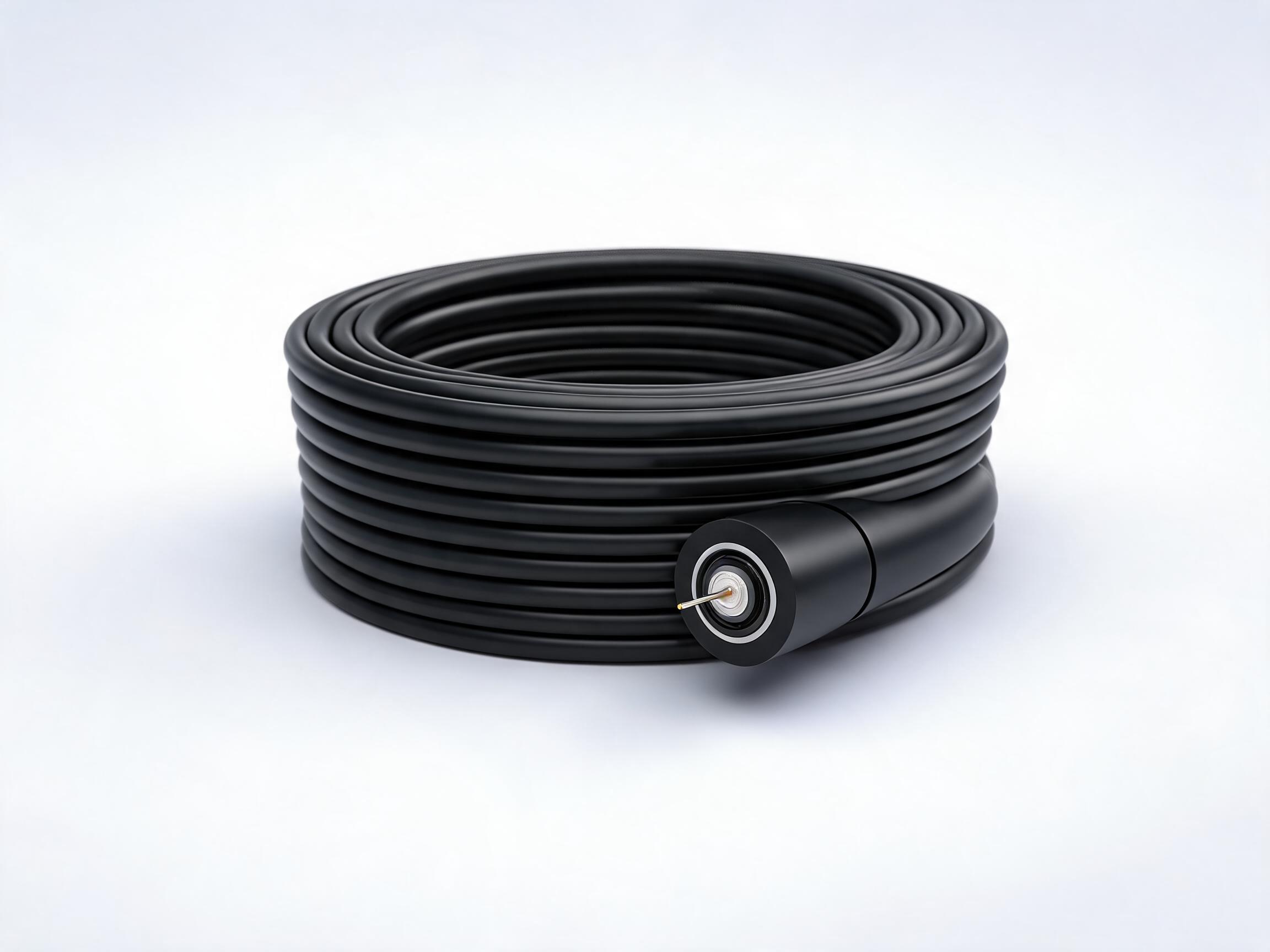
Where the route passes through ground with rodent activity, rocky backfill or recurring civil works, add armor: an armored fiber optic cable places a corrugated steel tape between the core and the jacket, which converts a shovel nick or a rodent bite from a fiber-damaging event into a jacket-level event. Armor costs more per meter than a non-armored build, and it is cheap insurance on exactly the sections where excavation damage is likely.
Aerial routes on existing poles: self-supporting constructions
Surveillance routes along roads and perimeters often follow pole lines that already carry power or telecom cables, and stringing a new duct along that corridor is rarely economical. Two aerial constructions solve the problem in different situations. A figure-8 self-supporting cable carries a suspended steel messenger integrated into the same sheath as the optical core, so the cable tensions itself; the installer lashes or clamps the messenger to the poles and the optical core rides below it. This is the fastest aerial method on short and medium spans between light poles and utility poles.
Where the route runs parallel to medium-voltage power lines or crosses energized railway infrastructure, a fully dielectric ADSS (All-Dielectric Self-Supporting) cable is the safer choice: it contains no metallic parts, so it neither conducts induced voltage nor requires grounding along the span, and it is designed to support itself over long spans under controlled tension. The trade-off is that ADSS requires a tension and sag calculation for each span, which is why the figure-8 construction usually wins on simple, short urban pole lines and ADSS wins on long or electrically exposed spans. We cover both constructions in depth in the deployment guides for figure-8 aerial cable and ADSS aerial selection.
Inside buildings: distribution and tight-buffered cable
The final meters of the backbone — from the building entry point to the control-room frame — run indoors, where the requirements change: smaller bending spaces, fire-code considerations for the jacket, and frequent handling at patch frames. A distribution fiber optic cable packs several fibers under a compact jacket for this role, and tight-buffered constructions handle the short, frequently-handled runs inside racks. This indoor segment is short and inexpensive; specifying it as an afterthought with leftover outdoor cable is a common but avoidable mistake, because outdoor PE jacket is not permitted indoors in many building codes.
| Route Section | Recommended Construction | Watch-Outs |
|---|---|---|
| Long buried corridor along a fence or road | Outdoor G.652D loose tube, 2-288 cores, black PE | Depth below local frost line with bedding; verify route against future excavation plans. |
| Buried through rodent or rocky ground | Armored outdoor cable (steel tape armor) | Armor is conductive; plan grounding at closures where required. |
| Duct run between buildings on one site | Outdoor loose tube or armored, sized to the duct | Confirm duct inner diameter and pulling distances before ordering drum lengths. |
| Aerial span between light poles, no power line conflict | Figure-8 self-supporting cable | Clamp or lash the messenger properly; keep sag within design limits. |
| Aerial parallel to MV power lines or rail | ADSS all-dielectric self-supporting | Span tension and sag calculation per span; hardware must match the cable. |
| Building entry to control-room frame | Distribution or tight-buffered indoor cable, LSZH where required | Confirm local fire code on jacket type; label both ends. |
How to Plan Fiber Count for a Camera Route
Fiber count is the decision that is hardest to change after installation, so it deserves more analysis than any other parameter on the schedule. The planning question is not "how many cameras do I have today" but "how many optical segments will this route carry over its life".
Start from the architecture at the camera nodes. In a per-camera architecture, each camera link gets a dedicated fiber pair between the node and the control room; this suits small systems and critical cameras that must stay isolated. In an aggregated architecture, each camera cluster shares one or two fibers that feed a switch inside the node cabinet, and that switch aggregates 8 to 24 cameras onto the backbone; this is the standard design for anything above a few dozen cameras, and it multiplies the reach of every fiber you install.
With the architecture fixed, count the segments: a node with one aggregation switch typically consumes one or two fibers (transmit and receive, or a duplex pair), a ring or redundant path doubles that, and spare capacity covers the rest. Industry practice on municipal surveillance routes is to hold 30 to 50 percent spare fiber beyond the counted demand, because the cheapest time to add capacity to a route is the day you order the cable. A 48-core cable serving 20 camera nodes today leaves room for node additions, a second control center, or traffic from other departments — fiber strands cost little extra at order time and are impractical to retrofit through a finished duct.
Core counts from 2 to 288 are available on the outdoor construction referenced above, so the cable schedule can be matched to each route section: a 12-core build suits a small access spur feeding four nodes, while a 144-core build serves the main spine that several distribution points share. We wrote a separate guide on choosing fiber count for a cable order that goes deeper into the counting method; the surveillance-specific rule is simply to count aggregation segments, add the redundancy you intend to build, and hold the spare percentage your organization's standards require.
Terminating Camera Nodes: Closures, Pigtails, and Slack
Between the cable drum and the camera sit the termination points where the field cable transitions into connectorized fiber: a pole-mounted or pedestal splice closure at each camera cluster, and a rack-mounted frame or wall box inside the control room. This is where backbone quality is either preserved or thrown away, because the connector is the least repeatable component to build in the field.
The established practice is to keep every connector in the factory and every splice in the field. A fiber optic pigtail arrives with the connector already terminated, cured and polished on the production line, and leaves one bare fiber end for a single fusion splice onto the field cable. The splice is the operation a fusion splicer performs with a measurable, recorded result every day; field-installed connectors, by contrast, depend on a cleave angle, a polish and a ferrule handled in a dusty cabinet, which is why links terminated entirely in the field show a wider spread of insertion-loss readings at acceptance. Factory-terminated pigtails are specified at 0.3 dB typical and 0.5 dB maximum insertion loss (1310/1550 nm), with return loss of 50 dB or better for UPC and 60 dB or better for APC end faces — figures measured on the finished assembly before packing, and the figures your acceptance test should compare against.
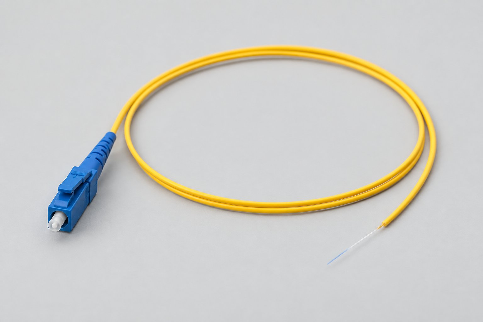
At the node cabinet, the working sequence is: land the outdoor cable in the closure, splice each needed fiber to a pigtail, store the splice protectors and slack in the closure tray, and leave the pigtail connector accessible inside the cabinet for the short cord that reaches the media converter or switch. Match the pigtail connector to the panel and active equipment — SC where cabinet space is comfortable, LC where the node cabinet is compact and port density matters. Confirm the end face (UPC or APC) together with the transceivers, not separately: mixing polish types in one path is a documented cause of reflectance problems, covered in the section on control-room connections below.
Slack handling at the node deserves its own line in the method statement. Every closure should hold enough stored cable to let the closure be reopened and the splices re-made at ground or pole level without re-pulling cable, and the slack coils must respect the cable's minimum bend radius — typically 20 times the cable diameter during installation and 10 times in service for the loose-tube constructions referenced here. We cover closure selection and slack storage in a dedicated guide on splice closures and slack management; the surveillance-specific point is that camera nodes are exactly the locations where future re-entry is likely, because cameras are re-aimed, replaced and added throughout the system's life.
Control Room and Cabinet Connections: Patch Cords and Adapters
Inside the control room and the aggregation cabinets, the backbone becomes a patching problem: the terminated fibers from the field land in an ODF or patch panel, and short factory-made cords connect them to the converters and switches. Two components do this work, and both are ordered by the same logic as the pigtails — match the connector, the polish and the fiber to the equipment at both ends of each link.
Patch cords: the last two connectors on every camera link
An SC-SC single mode G.652D patch cord (or its LC equivalent) carries the link from the ODF port to the media converter or switch transceiver. Its specification matters because the two mated pairs it creates are part of every camera link's loss budget: insertion loss is specified at 0.5 dB maximum per cord (release limit) with 0.3 dB as the typical production value, and return loss follows the polish — 50 dB or better for UPC, 60 dB or better for APC. Cords are available simplex or duplex, in LSZH or PVC jacket with 2.0 or 3.0 mm outer diameter, in custom lengths from 0.5 to 30 meters, so each position can be ordered to the actual path length instead of coiling excess cord behind the frame.
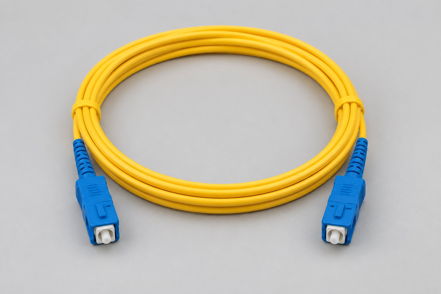
The polish decision belongs to the link, not to the component. UPC and APC ferrules are not interchangeable — mating a UPC cord into an APC port leaves an air gap at the core that degrades return loss by 10 to 20 dB below the specified level, and the fault is invisible at a quick continuity check. On a surveillance network the rule is simple: keep one polish family per optical path, end to end, and record the polish type in the port labeling so the next contractor's cord order matches.
Adapters: small parts that hold the mated pair on specification
Every cord plugs into an adapter, and the adapter's alignment sleeve is what keeps the two ferrules centered and in physical contact. An LC/UPC duplex fiber optic adapter with a precision zirconia sleeve is specified at 0.2 dB typical insertion loss and 50 dB or better return loss for UPC polish at 1310/1550 nm — values that hold only when the end faces entering the adapter are clean. The duplex body keeps a transmit/receive pair in one housing, which halves the cutouts in a panel and keeps port labeling unambiguous during moves, adds and changes. Adapters come flanged (fixed in a panel cutout) or unflanged (pressed into a holder for modular layouts); match the flange type to the panel you are filling.
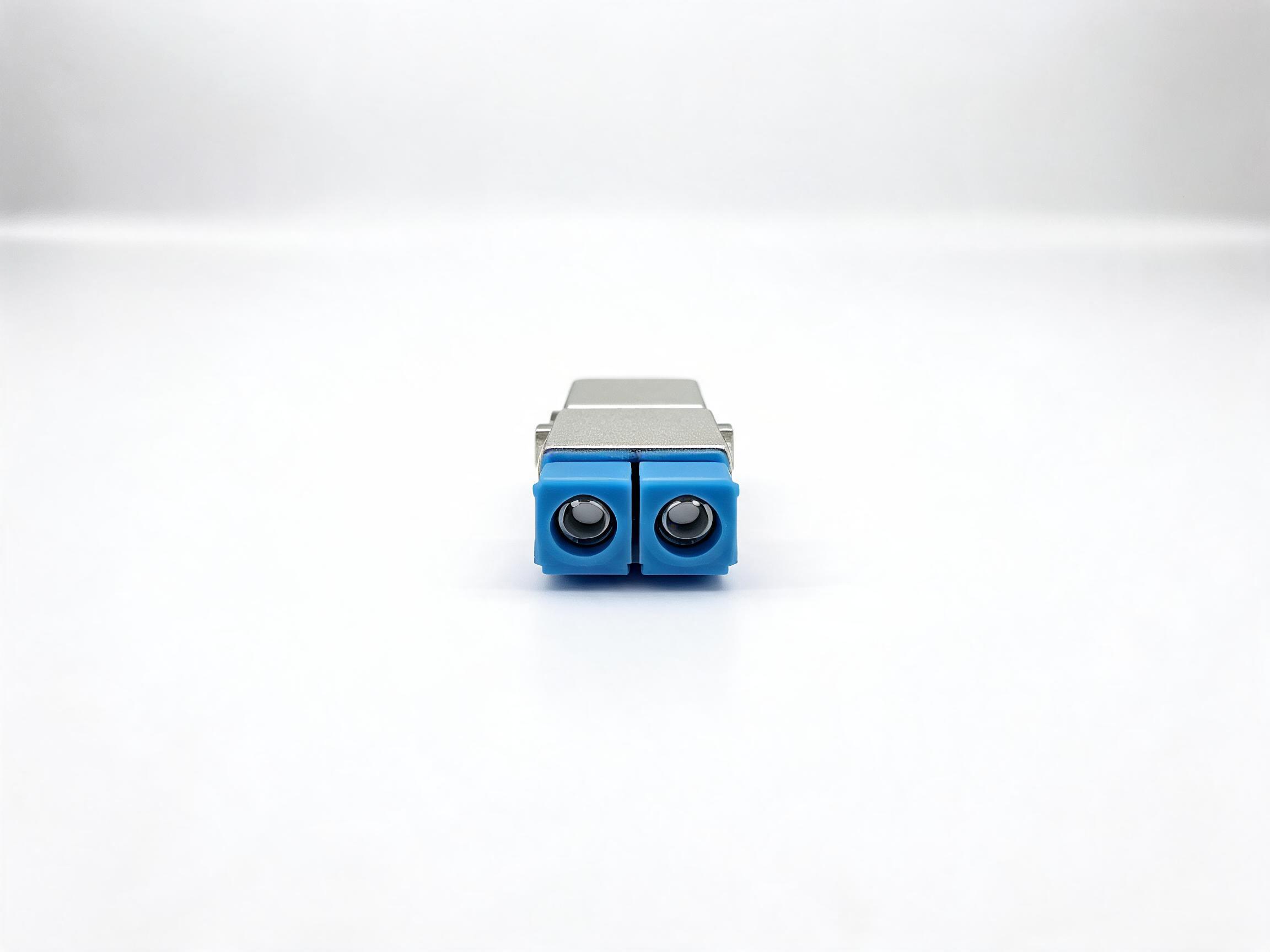
Two handling rules protect these numbers in practice. First, keep dust caps on connectors until the moment of mating, and clean and inspect end faces before every re-patch — a contaminated end face is the most common cause of a return-loss reading below specification. Second, after a large re-patching cycle, re-check insertion loss on a sample of ports rather than assuming the panel is unchanged. The full set of reading figures for cords and their meaning is explained in our guide to reading patch cord specifications.
Checking the Link Budget on a Surveillance Route
Before any hardware is ordered, the longest optical path in the design should pass an arithmetic check: do the transceivers at both ends have enough optical budget to cover everything the route consumes? The calculation takes ten minutes and prevents the most expensive class of surveillance-network failure — a backbone that was installed complete and then fails acceptance on the longest leg.
List the losses in order. Fiber attenuation on the referenced outdoor construction is typically 0.36 dB/km at 1310 nm and 0.22 dB/km at 1550 nm, so an 8-kilometer buried section consumes roughly 2.9 dB at 1310 nm and 1.8 dB at 1550 nm from fiber alone. Each fusion splice adds a typical 0.1 dB; a route with two mid-span closures carries four splices, about 0.4 dB. Each mated connector pair adds up to the cord and adapter specifications above — a conservative planning figure of 0.5 dB per mated pair covers the patch cord release limit, and the adapters' 0.2 dB typical value sits inside the mated-pair allowance. Add a spares-and-aging margin of 1 to 3 dB for future splices, cable repairs and connector wear, then compare the total against the optical budget of the selected transceivers, which ranges from a few decibels on short-reach optics to well over 20 dB on long-reach models.
A worked example shows how much headroom a typical route keeps. An 8-kilometer camera corridor with two closures, terminated with pigtails at both ends and connected through patch cords at the ODF and the node cabinet, consumes approximately 2.9 dB (fiber) + 0.4 dB (splices) + 2.0 dB (four mated pairs) + 2.0 dB (margin) = 7.3 dB at 1310 nm. Almost every single mode transceiver on the market clears this comfortably, which is the point: the budget check exists to catch the exceptional route — the 40-kilometer highway segment, the daisy-chained corridor with six closures — before it is ordered. The full method, with a fill-in table, is in our guide to calculating a fiber optic link loss budget.
After installation, verify the arithmetic rather than trusting it. An insertion-loss test with a light source and power meter at 1310 and 1550 nm compares the as-built route against the calculated budget, and an OTDR trace documents the fiber's condition along its length for the maintenance file. We describe both procedures in the guides to insertion-loss testing with a light source and power meter and OTDR acceptance testing. All attenuation and loss values in this section are industry typical values; the specification sheet issued with your order is the authoritative reference for the product you receive.
Deployment Notes That Protect the Backbone
The cable constructions referenced in this article carry published installation limits, and most surveillance-route damage traces back to three of them: bend radius, pulling tension and sealing.
Bend radius is the easiest to violate and the easiest to protect. For the loose-tube outdoor constructions referenced here, typical limits are 20 times the cable diameter during installation and 10 times in service — figures to confirm on the datasheet for the exact build. At a 12-millimeter cable diameter, that is a 240-millimeter radius while pulling and 120 millimeters once the cable is landed. Slack coils in closures, cable transition boxes and control-room entries are where installers meet these limits repeatedly; a coil pulled tight around a fixture corner can add measurable attenuation that a final link test will attribute to the route as a whole.
Pulling tension is managed the same way as on any backbone route: keep the winch below the cable's short-term tensile limit — 1,500 N short-term for the smaller core counts of the referenced outdoor construction, rising with core count — monitor it with a dynamometer, and use a swivel to prevent twist. Cable lubricant on long duct runs and a mid-assist pull on runs approaching the tension limit are cheaper than a re-pull. The contractor-facing details, including dynamometer setup and lubricant selection, are covered in our guide to pulling cable without exceeding tension and bend limits, and the buried-route details — depth, bedding and backfill — are in the guide to direct-buried installation.
Sealing completes the protection: every closure and building entry must be sealed per its design, because water is the slow failure mode of outdoor plant. The referenced outdoor cable carries an operating temperature range of -40 °C to +70 °C as a typical value, which covers pole-mounted closures in most climates; verify against the datasheet for installations in extreme environments.
Common Design Mistakes in Surveillance Fiber Projects
Reviewing surveillance projects that ran into trouble after commissioning, the same handful of design mistakes recurs. None of them is exotic, and all of them are cheaper to prevent during the design phase.
- Polish mismatches left in the plant. A UPC cord patched into an APC port passes a continuity check and fails a reflectance test. Decide the polish family per link, label it at both ends, and order pigtails, cords and adapters to match.
- No spare fiber. Counting exactly today's demand turns every camera addition into a new construction project. Hold 30 to 50 percent spare on backbone routes.
- Mixed fiber grades at a splice. A multimode pigtail spliced to a single mode field cable will show high and unstable loss. Keep fiber grades consistent across each optical path and check them when pigtails are ordered.
- Unplanned node power. Aggregation switches and converters at camera nodes need power; discovering at commissioning that the pole cabinet has none is a schedule problem, not a fiber problem. Design node power alongside the cable schedule.
- Slack coiled beyond bend limits. Excess cord and cable coiled tightly inside cabinets adds loss that surfaces as an unexplained link-budget shortfall at acceptance.
- No as-built documentation. Port labels, fiber maps and test records are what let the next contractor add a camera without re-testing the entire backbone. Specify the documentation deliverable in the installation contract.
How the Backbone Grows: Three Expansion Scenarios Worth Designing For
A surveillance backbone that was designed only for opening day will be re-purchased at the first expansion. Three growth patterns account for most of the change orders we see on camera projects, and each one costs almost nothing if the passive plant anticipated it.
Camera additions at existing nodes. This is the most common change: a cluster grows from 8 to 16 cameras, or a new ANPR lane appears at a gate. The backbone fibers are already in the node cabinet — the work is a new switch port, a spare pair from the closure tray, and a short cord. The design requirement is simply that the closure was sized for the splices and that spare fibers were left landed and labeled at the panel, which is why the spare-fiber rule in the fiber-count section matters more than any other single figure in this article.
New nodes on existing routes. A route that passes within reach of a new parking area or building entrance can pick up a node without new construction if the cable schedule left slack loops at planned intervals. This is a method-statement decision, not a product decision: instruct the installer to land a slack loop at each future node location, protected in a closure or handhole, and the marginal cost of the next node drops to a closure, a converter and labor.
Service growth on spare fibers. The spare strands designed into the backbone eventually carry traffic that did not exist when the cable was ordered — environmental sensors, public Wi-Fi backhaul, perimeter analytics for a neighboring facility, or a second operator leasing dark fiber. Because the fibers were ordered and installed in one civil-works campaign, the incremental cost of serving each of these is a termination, not a trench. Integrators who hold the as-built fiber map and port documentation can quote these add-ons in days; projects without documentation have to re-locate fibers with an OTDR before anyone can promise the spare capacity.
The pattern across all three scenarios is the same: the backbone's value at year five is determined by decisions made at order time — spare core count, slack at planned intervals, and documentation that survives staff turnover. None of them adds meaningful cost to the initial order; all of them are expensive to retrofit.
What to Verify with Your Cable Supplier Before the Order
The passive plant of a surveillance backbone is ordered once and expected to run for the life of the system, so the supplier conversation should cover manufacturing quality, delivery and after-sales support with the same seriousness as the technical specification.
Manufacturing and quality control
Nexora Communications has manufactured fiber optic connectivity products in Shenzhen since 2014. The facility covers 16,000+ square meters with 180+ employees and 12 production lines, and quality control runs through the whole process across 30+ QC stations covering incoming material, component, in-process, functional, visual, final and packaging inspection. Cable production capacity is stated at 2.8M+ units per year and 230K+ units per month across the product range, with more than 3,500 configurations in production. Every reel of outdoor cable is tested for attenuation and continuity before dispatch, and the test report can be supplied with the shipment on request — a detail worth requesting in writing, because it is the document your acceptance team compares against. These are company-level manufacturing facts describing the factory behind the products referenced in this article, not product-specific certifications.
Commercial terms to confirm in writing
Minimum order quantities and lead times differ by product family, and knowing them before finalizing the design keeps the procurement schedule realistic:
| Product | Typical MOQ | Typical Lead Time |
|---|---|---|
| Outdoor G.652D single mode cable | Typically from 10 km per order for standard core counts; custom configurations quoted separately | 15-20 working days for standard configurations |
| Fiber optic pigtails | 100 pcs per configuration | 7-15 working days for standard configurations |
| SC-SC single mode patch cords | 100 pcs per configuration | 7-15 working days; 15-25 for mixed or high-volume orders |
| LC/UPC duplex adapters | 1,000 pcs for standard configurations | 7-15 working days for standard orders |
Cable is supplied on wooden drums in standard lengths of 2, 4 and 6 km, wrapped in moisture-barrier film and secured with steel strapping; drum lengths should be planned against the route's splice-point spacing so that mid-route drums are not opened unnecessarily. Custom jacket printing and custom drum lengths are available for OEM and ODM orders — useful on municipal projects where the cable owner requires the route identifier printed on the jacket. Standard payment terms are T/T, commonly 30% deposit with the balance before shipment, with L/C accepted for larger orders; the applicable terms are stated on the proforma invoice.
Warranty
All Nexora fiber optic cables and connectivity products referenced in this article carry a 12-month warranty from shipment date, covering manufacturing defects. A claim is raised by sending the batch or reel reference, the affected quantity and a test record showing the measured value; confirmed manufacturing defects are replaced or credited, with a response within 5 working days and replacement stock typically dispatched within 15 working days of claim confirmation. Damage caused during installation, by third-party civil work, or by use outside the specified operating conditions is outside the warranty scope — one more reason to keep the installation method statement and the as-built test records organized from day one.
Frequently Asked Questions
How many fibers do I need for 100 cameras?
Count aggregation segments, not cameras. With node cabinets each aggregating 16 cameras on a duplex fiber pair, 100 cameras need roughly 7 node links — 14 fibers — plus a redundant path and 30-50% spare, which lands most designs on a 24- or 48-core backbone cable. The right number depends on your node layout and redundancy plan, which is why it should be calculated per route rather than copied between projects.
Do surveillance links need APC or UPC connectors?
Either works optically for digital video links; what matters is consistency. Keep one polish family across each optical path — pigtails, cords, adapters and transceivers — and follow whatever your organization's standard specifies. APC offers higher return loss (60 dB or better versus 50 dB for UPC), which matters most on analogue video or RF-overlay services; digital IP video links commonly run UPC throughout.
Can one fiber carry several cameras?
Yes, and that is exactly what the aggregated architecture does: a switch at the camera node combines many camera streams onto one or two backbone fibers. The backbone carries the aggregate bandwidth; with modern optics a single fiber pair has far more capacity than any realistic camera cluster produces.
What cable should connect buildings across one campus?
For ducted or buried campus links, the same outdoor loose-tube G.652D construction used on long routes is the right answer, with core count sized to the number of buildings and services sharing the duct. For campus runs between buildings where indoor jacket is required, confirm the fire code transition point with the building entry — outdoor cable transitions to indoor distribution cable at a controlled entry point, not gradually along the corridor.
Can the same backbone carry other services besides CCTV?
Yes — and spare fibers are designed for exactly this. Traffic-light data, public Wi-Fi backhaul, environmental sensors or intercom systems can ride on spare strands of the same cable. This is the strongest argument for ordering spare capacity: the marginal cost of extra fibers at order time is small compared with a second cable pull later.
What documentation should come with a cable order?
At minimum: the specification sheet for the exact configuration ordered, factory test reports for attenuation and continuity per reel (requested in advance), packing lists with drum numbers, and batch references on connectivity packaging that let any claim trace back to the production record. Confirm the document format during quotation so it arrives with the goods rather than after.
How do I raise a warranty claim on a defective component?
Send the batch or reel reference printed on the packaging, the affected quantity, and a test record showing the measured value within the claim window. Confirmed manufacturing defects are replaced or credited; the process and timelines are described in the warranty section above, and keeping the original packaging labels until incoming inspection is complete is what makes the trace possible.
Plan Your Surveillance Backbone With Nexora
A CCTV backbone is a one-time investment in the transmission layer of a system that will be expanded, re-patched and relied upon for years. If you are planning a surveillance project, send us the route description — buried, ducted or aerial sections and their lengths, the number of camera nodes, the fiber counts you have calculated, and the connector and polish your equipment requires — and we will confirm the cable constructions, core counts, drum lengths and connectivity package that match, together with lead times and a quotation. Short cable samples for evaluation are available, and test documentation travels with the order on request.